Complex functions plotting

Complex Functions Plotting

Plotting in 1D

Plotting in 2D

Introduction

When creating physics simulations, especially in the realm of quantum mechanics and classical wave phenomena, dealing with complex functions is a common necessity. Visualizing these complex functions effectively is crucial for understanding their behavior and properties.

This guide will cover two approaches for visualizing complex functions in one dimension:

1. Plotting Real and Imaginary Parts Separately: This method involves plotting the real part and the imaginary part of the complex function as separate curves on the same graph.
2. Hue and Magnitude Scheme: In this approach, the magnitude of the complex function is shaded below with a hue determined by the phase. This provides a comprehensive visual representation of both magnitude and phase.

For visualizing complex functions in two dimensions, we will use the hue scheme exclusively, as it is particularly effective in conveying the intricate details of complex functions across two spatial dimensions.

Let’s explore each method with examples and plots to illustrate these concepts.

Plotting in 1D

In physics simulations, especially in quantum mechanics, a wavepacket is a common entity used to represent localized particles. A wavepacket is essentially a localized wave that can be described by a Gaussian function modulated by a complex exponential. This combines both position and momentum information, making it an ideal representation for quantum states.

Here, we create a wavepacket using the following steps:

1. Gaussian Shape: We start with a Gaussian function centered at x_0 with a standard deviation \sigma. This represents the spatial localization of the wavepacket.
2. Wave Component: We modulate this Gaussian by a complex exponential term e^{-i p x / \hbar}, where p is the momentum and \hbar is the reduced Planck’s constant. This adds the momentum component to the wavepacket.
3. Normalization: Finally, we normalize the wavepacket to ensure it has a unit probability when integrated over all space.

import numpy as np

class Parameters:
    def __init__(self, x0, sigma, p, hbar, dx):
        self.x0 = x0
        self.sigma = sigma
        self.p = p
        self.hbar = hbar
        self.dx = dx

p = Parameters(x0=0, sigma=1, p=1, hbar=1, dx=0.01)

def create_wavepacket(x):
    # Gaussian shape
    gaussian = np.exp(-(x - p.x0) ** 2 / (2 * p.sigma ** 2))
    # Adding the wave component (momentum)
    psi0 = gaussian * np.exp(-1j * p.p * x / p.hbar)
    # Normalize
    psi0 /= np.sqrt(np.sum(np.abs(psi0) ** 2) * p.dx)
    return psi0

x = np.arange(-10, 10, p.dx)
psi = create_wavepacket(x)

To visualize the complex wavepacket, we use three different methods:

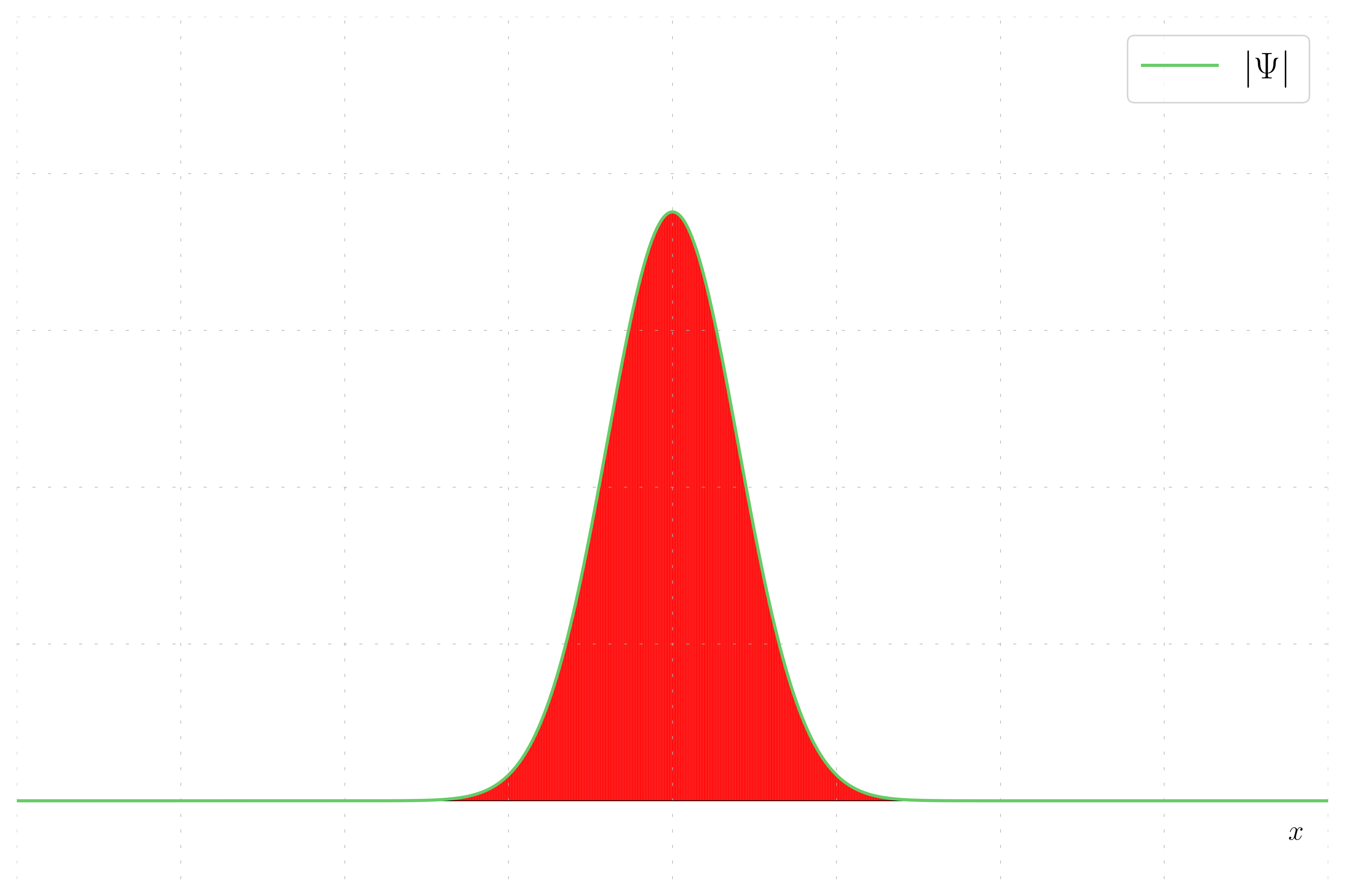
1. Probability Density: This method involve plotting the probability density. This show the probability to find the particles when making measurements.

2. Plotting Real and Imaginary Parts Separately: This method involves plotting the real part and the imaginary part of the wavepacket separately on the same graph. This helps in understanding the individual contributions of the real and imaginary components.

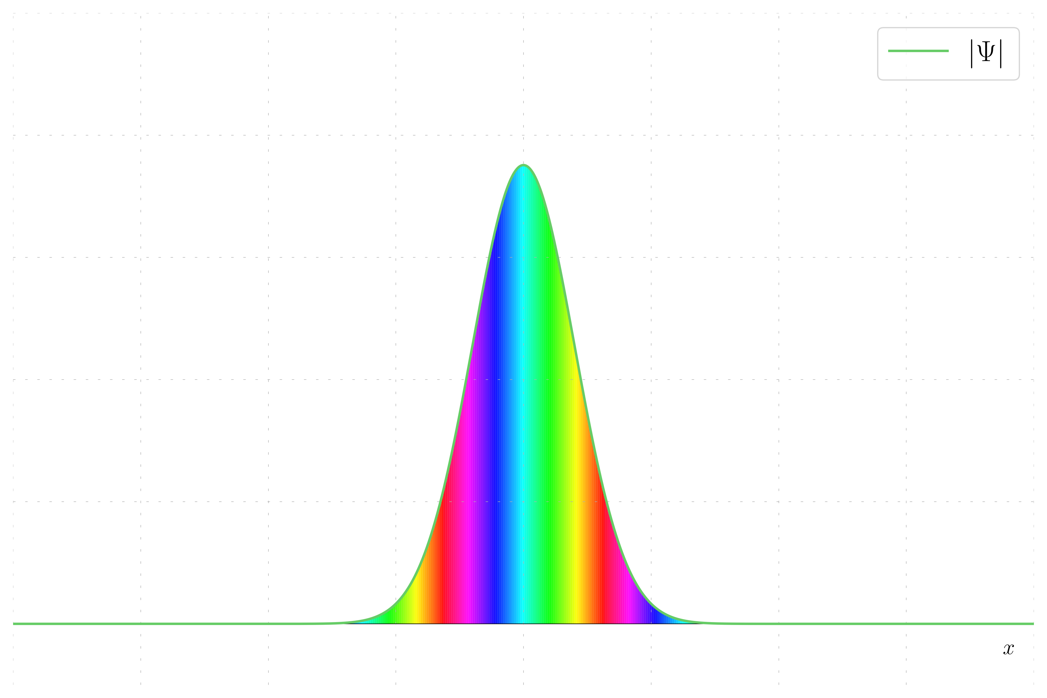
3. Hue and Magnitude Scheme: This method uses color to represent the phase of the complex wavepacket and shading to represent the magnitude. The phase is mapped to a hue, while the magnitude determines the brightness, providing a comprehensive view of both aspects of the wavepacket.

import matplotlib.pyplot as plt
from matplotlib.collections import PolyCollection

# Define colors
class Colors:
    def __init__(self):
        self.r = 'red'
        self.b = 'blue'
        self.o = 'orange'
        self.g = 'green'

c = Colors()

# Plotting function
def plot_wavepacket(x, psi, plot_prob=True, plot_phase=False):
    fig, ax = plt.subplots()
    if plot_prob:
        line, = ax.plot(x, abs(psi.conjugate() * psi),
                        lw=2, color=c.r, label='$|\\Psi|^2$')
    else:
        if plot_phase:
            # Extract the phase of psi
            phase = np.angle(psi)
            # Normalize phase to [0, 1] for hsl
            normalized_phase = (phase + np.pi) / (2 * np.pi)
            # Create vertices for PolyCollection
            polys = [np.column_stack([[x[j], x[j + 1], x[j + 1], x[j]], [0, 0, abs(psi[j + 1]), abs(psi[j])]]) for j in range(len(x) - 1)]
            poly = PolyCollection([], cmap='hsv', edgecolors='none')
            poly.set_verts(polys)
            poly.set_array(normalized_phase[:-1])
            ax.add_collection(poly)
        else:
            line1, = ax.plot(x, psi.real, lw=1.5, color=c.b, label='$\\Re\\{\\Psi\\}$')
            line2, = ax.plot(x, psi.imag, lw=1.5, color=c.o, label='$\\Im\\{\\Psi\\}$')
        line3, = ax.plot(x, abs(psi), lw=2, color=c.g, label='$|\\Psi|$')

    ax.legend()
    plt.show()

# Example usage
plot_wavepacket(x, psi, plot_prob=True)
plot_wavepacket(x, psi, plot_prob=False, plot_phase=True)
plot_wavepacket(x, psi, plot_prob=False, plot_phase=False)

To illustrate the concepts, let’s look at some specific examples of wavepackets:

• Probability Density: Shows how the probability of finding a particle varies with position.
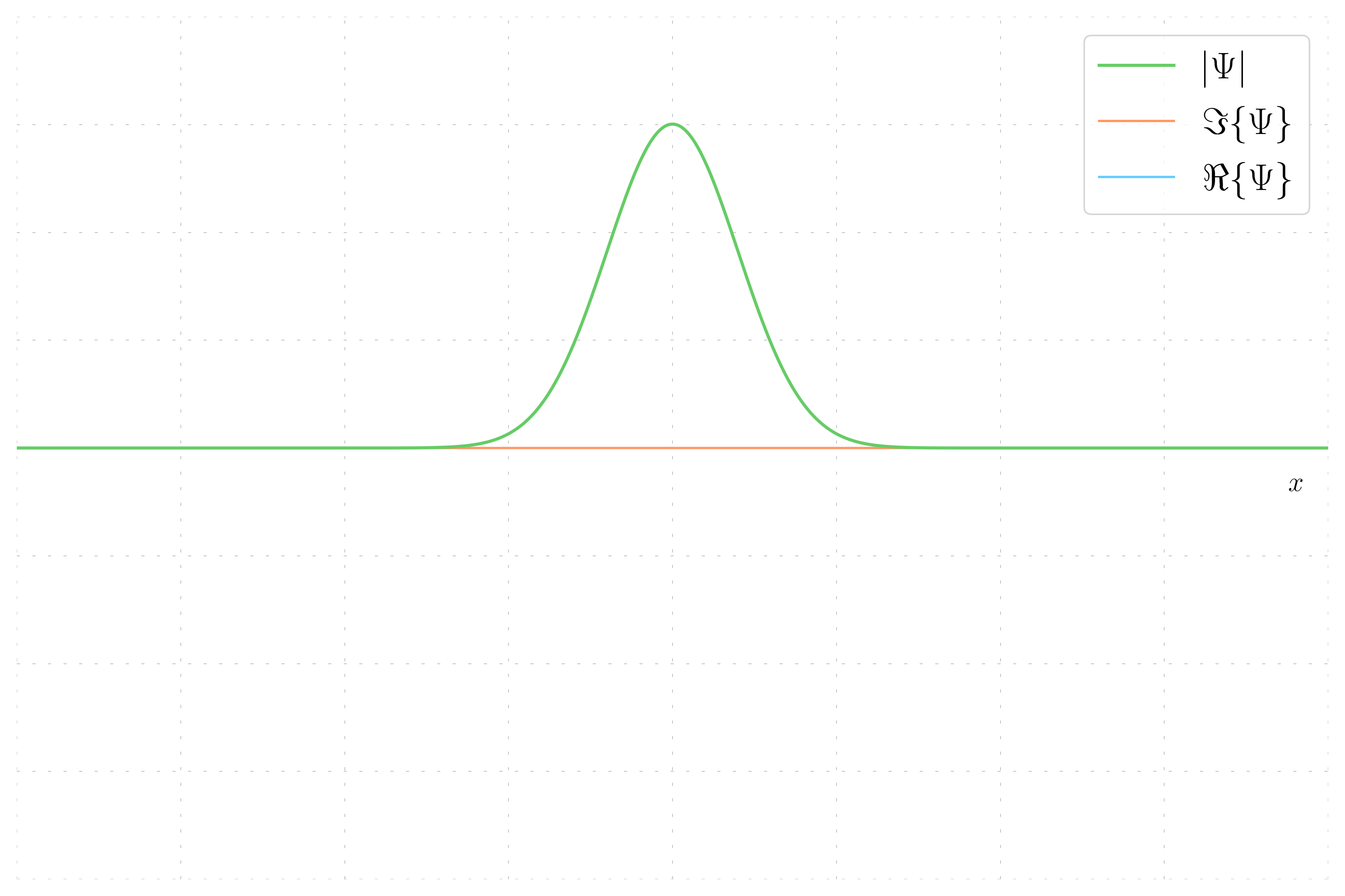
• Zero Momentum Wavefunction: The phase is constant, resulting in a uniform color, and the wavefunction equals its real part.
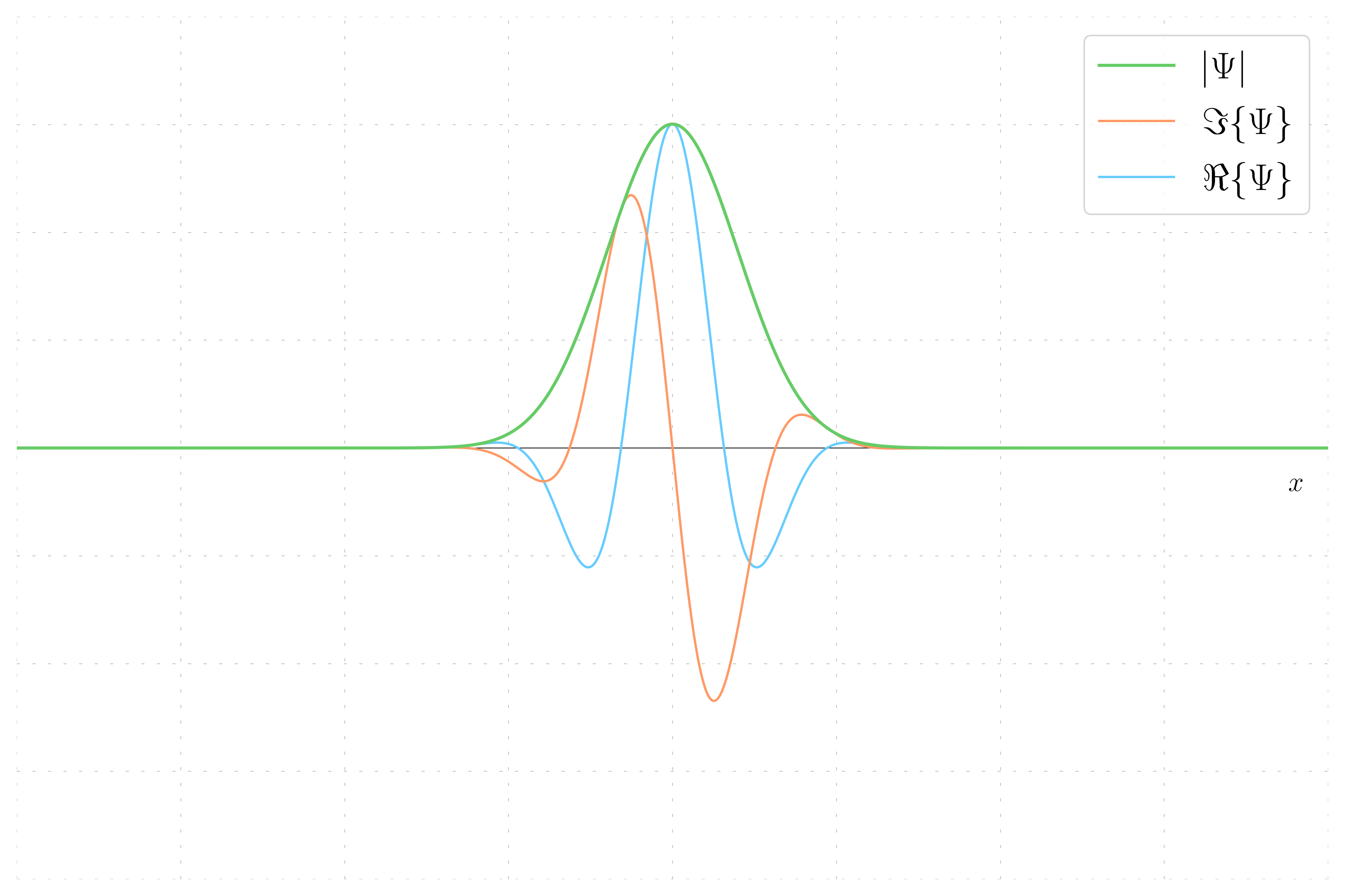
• Non-Zero Momentum Wavefunction: The phase varies, resulting in a striped hue pattern, and both real and imaginary parts are present due to the phase introduced by momentum.

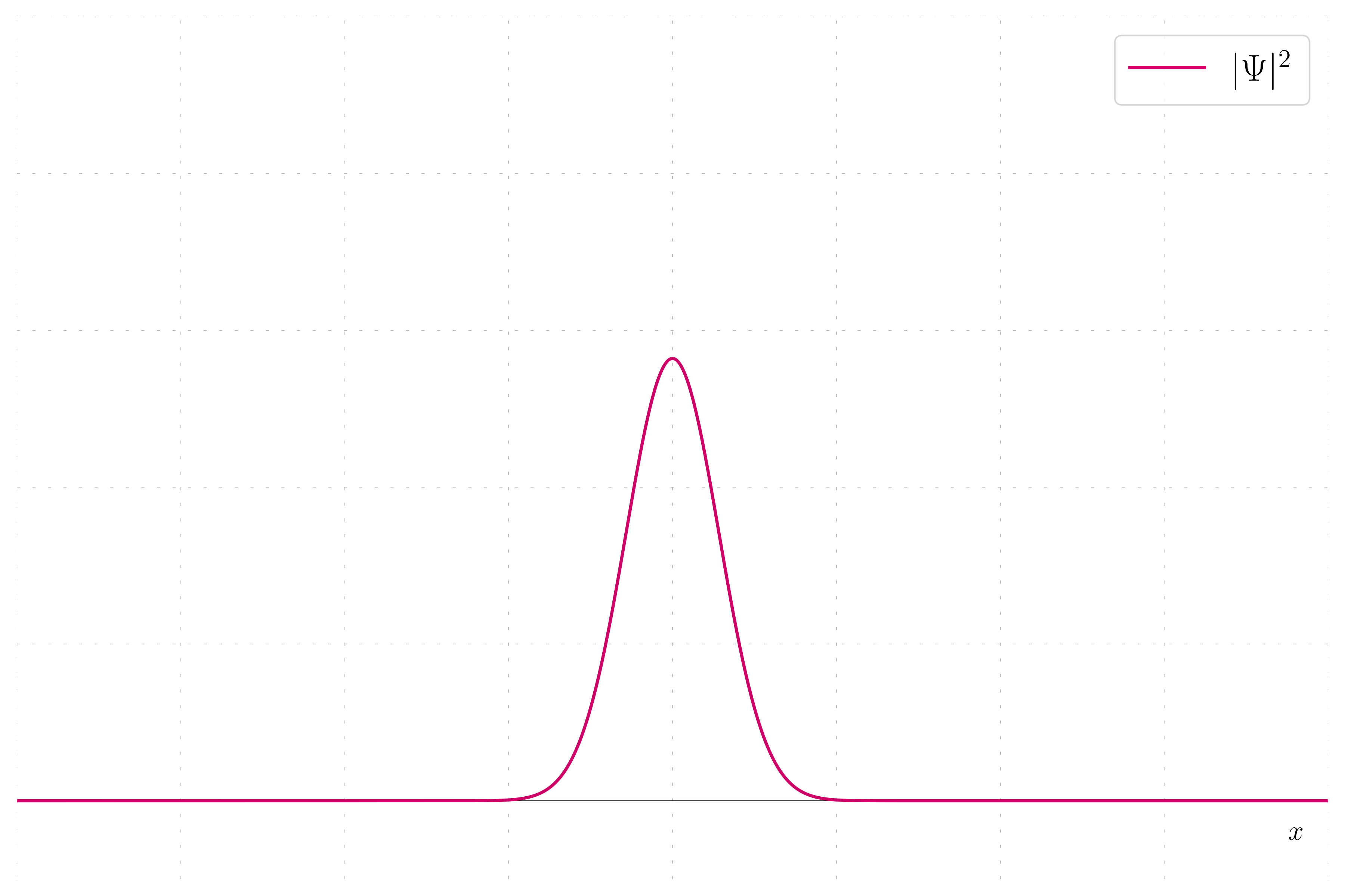
In quantum mechanics, the probability density of finding a particle at a given position is given by the squared magnitude of the wavefunction, |\psi|^2. This example plot the probability density of a wavepacket.

In this case, the wavepacket has no momentum, meaning the wavefunction is purely real and the imaginary part is zero. This results in the wavefunction being equal to its real part.

Here, the wavepacket has a non-zero momentum. The wavefunction now has both real and imaginary parts due to the phase introduced by the momentum.

To further illustrate the behavior of wavepackets, we will visualize the phase. The phase of the wavepacket is represented by different colors (hues). For a wavepacket with zero momentum, the phase remains constant, resulting in a uniform color. When the momentum is zero, the phase of the wavepacket remains constant, resulting in a uniform hue.

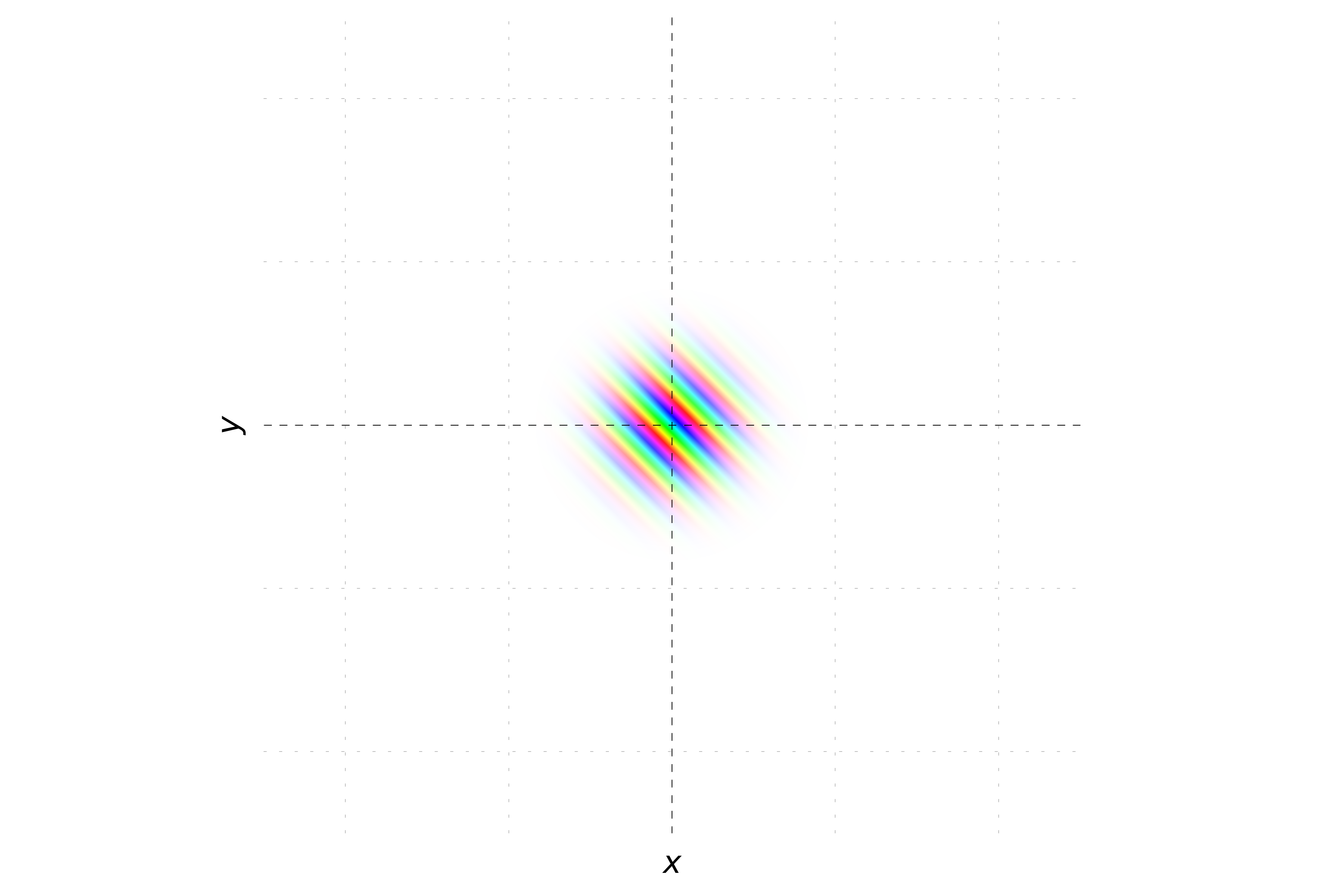
For a wavepacket with non-zero momentum, the phase varies linearly with position, creating a striped hue pattern.

Plotting in 2D

Similar to the 1D case, a 2D wavepacket can be constructed by extending the Gaussian and wave components into two dimensions. The 2D wavepacket is represented by a Gaussian function in both x and y directions, modulated by complex exponentials representing the momentum components in both directions.

import numpy as np

class Parameters2D:
    def __init__(self, x0, y0, sigma_x, sigma_y, p_x, p_y, hbar, dx, dy, xy_max, N):
        self.x0 = x0
        self.y0 = y0
        self.sigma_x = sigma_x
        self.sigma_y = sigma_y
        self.p_x = p_x
        self.p_y = p_y
        self.hbar = hbar
        self.dx = dx
        self.dy = dy
        self.xy_max = xy_max
        self.N = N

p2d = Parameters2D(x0=0, y0=0, sigma_x=1, sigma_y=1, p_x=1, p_y=1, hbar=1, dx=0.1, dy=0.1, xy_max=5, N=100)

def create_wavepacket_2d(X, Y):
    # Gaussian shape
    gaussian = np.exp(-(X - p2d.x0)**2 / (2 * p2d.sigma_x**2) - (Y - p2d.y0)**2 / (2 * p2d.sigma_y**2))
    # Adding the wave component (momentum)
    psi0 = gaussian * np.exp(1j * (p2d.p_x * X + p2d.p_y * Y) / p2d.hbar)
    # Normalize
    psi0 /= np.sqrt(np.sum(np.abs(psi0)**2) * p2d.dx * p2d.dy)
    return psi0

x = np.linspace(-p2d.xy_max, p2d.xy_max, p2d.N)
y = np.linspace(-p2d.xy_max, p2d.xy_max, p2d.N)
X, Y = np.meshgrid(x, y)
psi = create_wavepacket_2d(X, Y)

This code creates a 2D wavepacket with Gaussian spatial localization and complex exponential modulation to include momentum. The wavepacket is then normalized to ensure it has a unit probability when integrated over the entire 2D space.

To visualize the complex wavepacket in 2D, we use two different methods:

1. Probability Density: This method involves plotting the probability density. This shows the probability of finding the particles when making measurements.

2. Hue and Magnitude Scheme: This method uses color to represent the phase of the complex wavepacket and shading to represent the magnitude. The phase is mapped to a hue, while the magnitude determines the brightness.

Additionally, you can choose to plot in 2D or 3D.

def create_axes_3d(fig):
    ax = fig.add_subplot(111, projection='3d')
    ax.set_xlabel('X')
    ax.set_ylabel('Y')
    ax.set_zlabel('Probability Density')
    return ax

def create_axes_2d(ax):
    ax.set_xlabel('X')
    ax.set_ylabel('Y')

def plot_wavepacket(X, Y, psi, plot_3d=False, plot_prob=True):
    if plot_3d:
        fig = plt.figure(figsize=(12, 8))
    else:
        fig, ax = plt.subplots(figsize=(12, 8), dpi=300)
    plt.rcParams['text.latex.preamble'] = r"\usepackage{bm} \usepackage{amsmath} \usepackage{helvet}"
    plt.rcParams.update({"text.usetex": True, "font.family": "Helvetica", "font.sans-serif": "Helvetica"})

    if plot_3d:
        ax = create_axes_3d(fig)
    else:
        create_axes_2d(ax)



    if plot_prob:
        cmap = 'viridis'
        magnitude = abs(psi.conjugate() * psi)
        if plot_3d:
            mask = (abs(X) <= 3.2) & (abs(Y) <= 3.2)
            X_f = np.where(mask, X, np.nan)
            Y_f = np.where(mask, Y, np.nan)
            magnitude_f = np.where(mask, magnitude, np.nan)
            ax.plot_surface(X_f, Y_f, magnitude_f, cmap=cmap, rstride=1, cstride=1, linewidth=0, antialiased=False, shade=False)
        else:
            plt.pcolormesh(X, Y, magnitude, shading='auto', cmap=cmap, vmin=0, vmax=np.max(magnitude) * 1.05)
    else:
        magnitude = np.abs(psi)
        phase = np.angle(psi)
        normalized_phase = (phase + np.pi) / (2 * np.pi)
        hsv_image = cm.hsv(normalized_phase)
        if plot_3d:
            filtered_mask = magnitude < 1e-4
            hsv_image[filtered_mask] = [1, 1, 1, 1]  # RGBA for white
            mask = (abs(X) <= 5) & (abs(Y) <= 5)
            X_f = np.where(mask, X, np.nan)
            Y_f = np.where(mask, Y, np.nan)
            magnitude_f = np.where(mask, magnitude, np.nan)
            ax.plot_surface(X_f, Y_f, magnitude_f, facecolors=hsv_image, rstride=1, cstride=1, linewidth=0, antialiased=False, shade=False)
        else:
            hsv_image[..., 3] = np.clip(magnitude / np.nanmax(magnitude), 0, 1)
            ax.imshow(hsv_image, extent=(-5, 5, -5, 5), origin='lower')
    plt.tight_layout()
    plt.show()


# Example usage
plot_wavepacket(X, Y, psi, plot_prob=True, plot_3d=True)
plot_wavepacket(X, Y, psi, plot_prob=False, plot_3d=True)
plot_wavepacket(X, Y, psi, plot_prob=True, plot_3d=False)
plot_wavepacket(X, Y, psi, plot_prob=False, plot_3d=False)

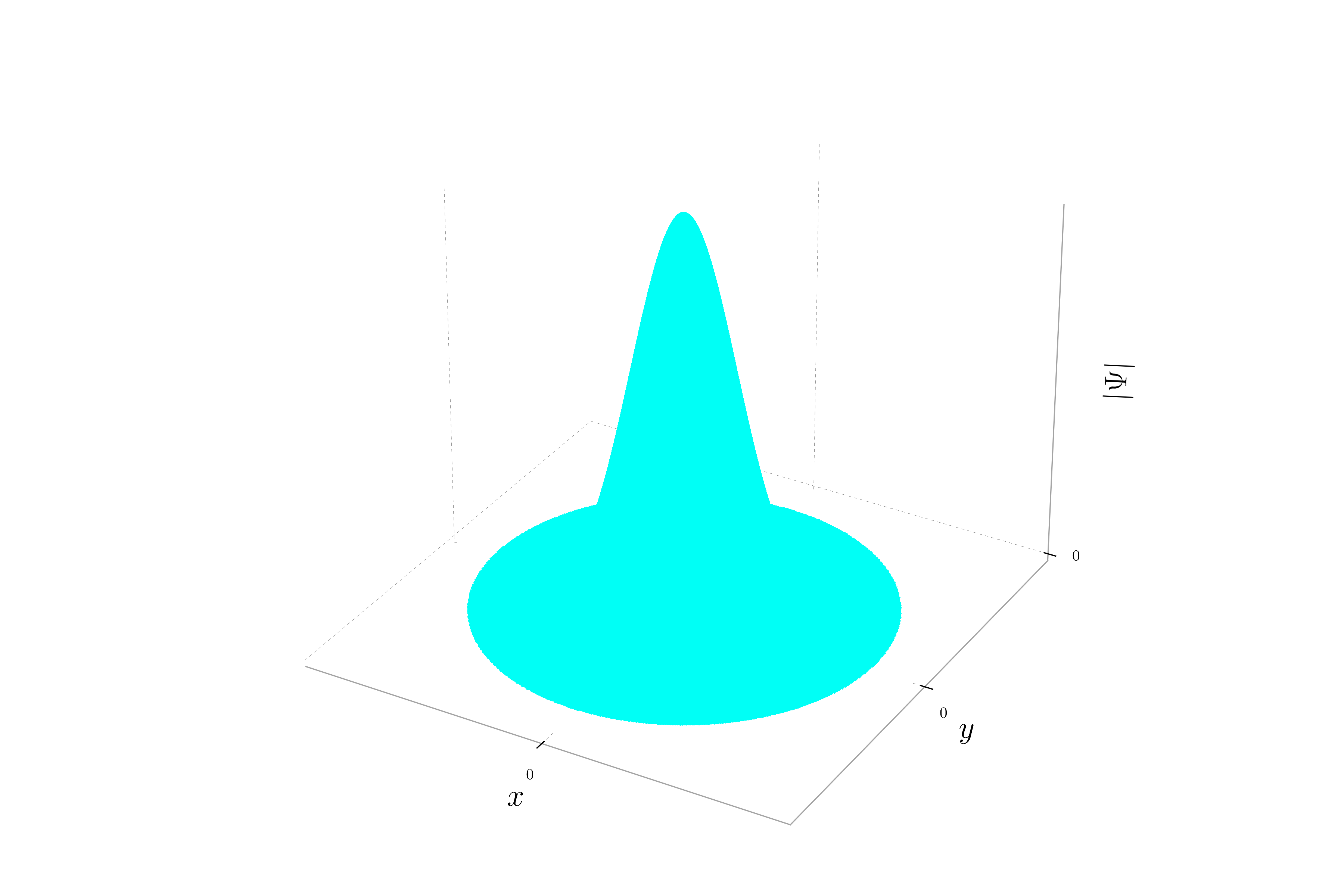
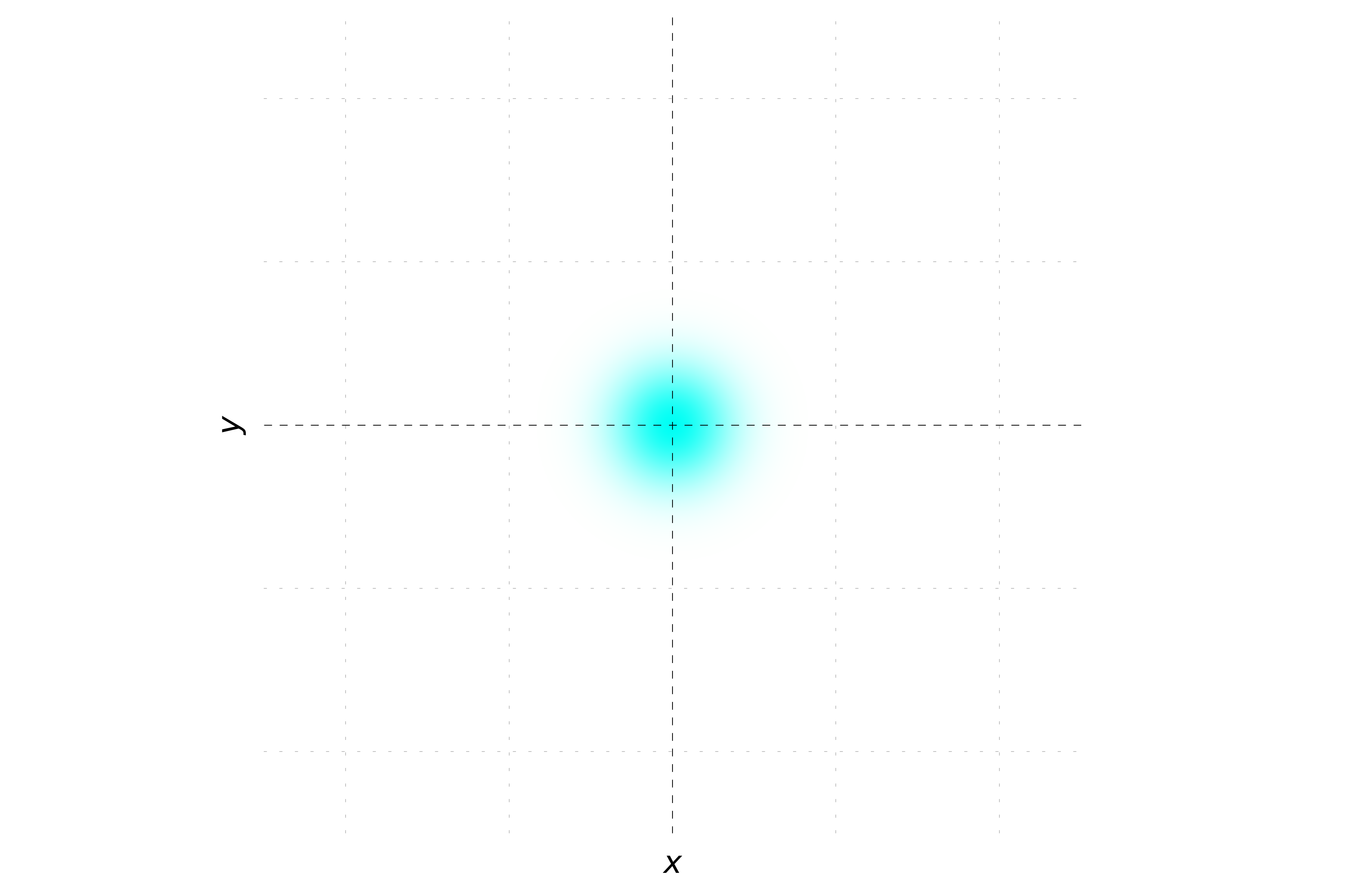
It is possible to plot the probability density.

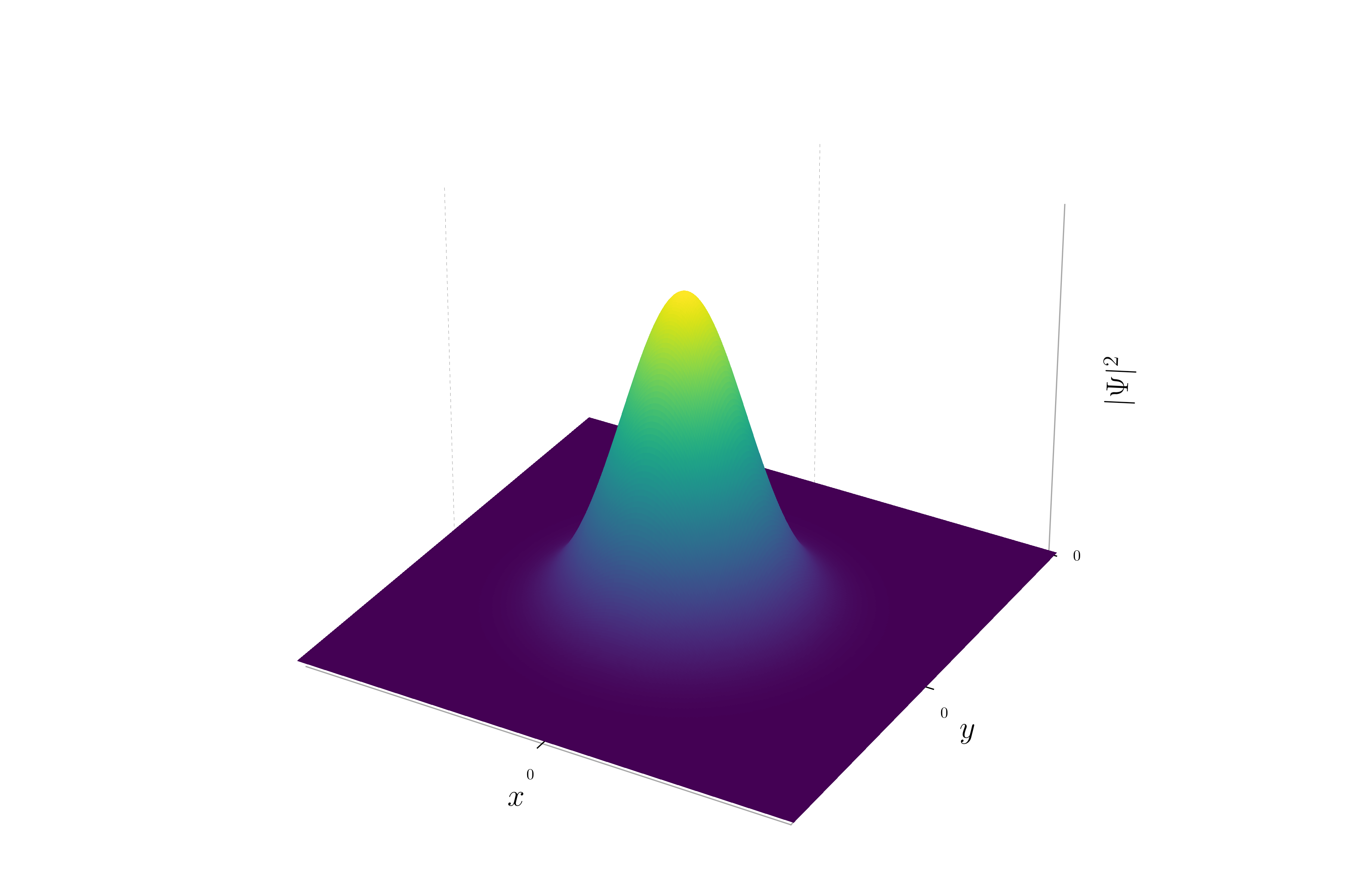
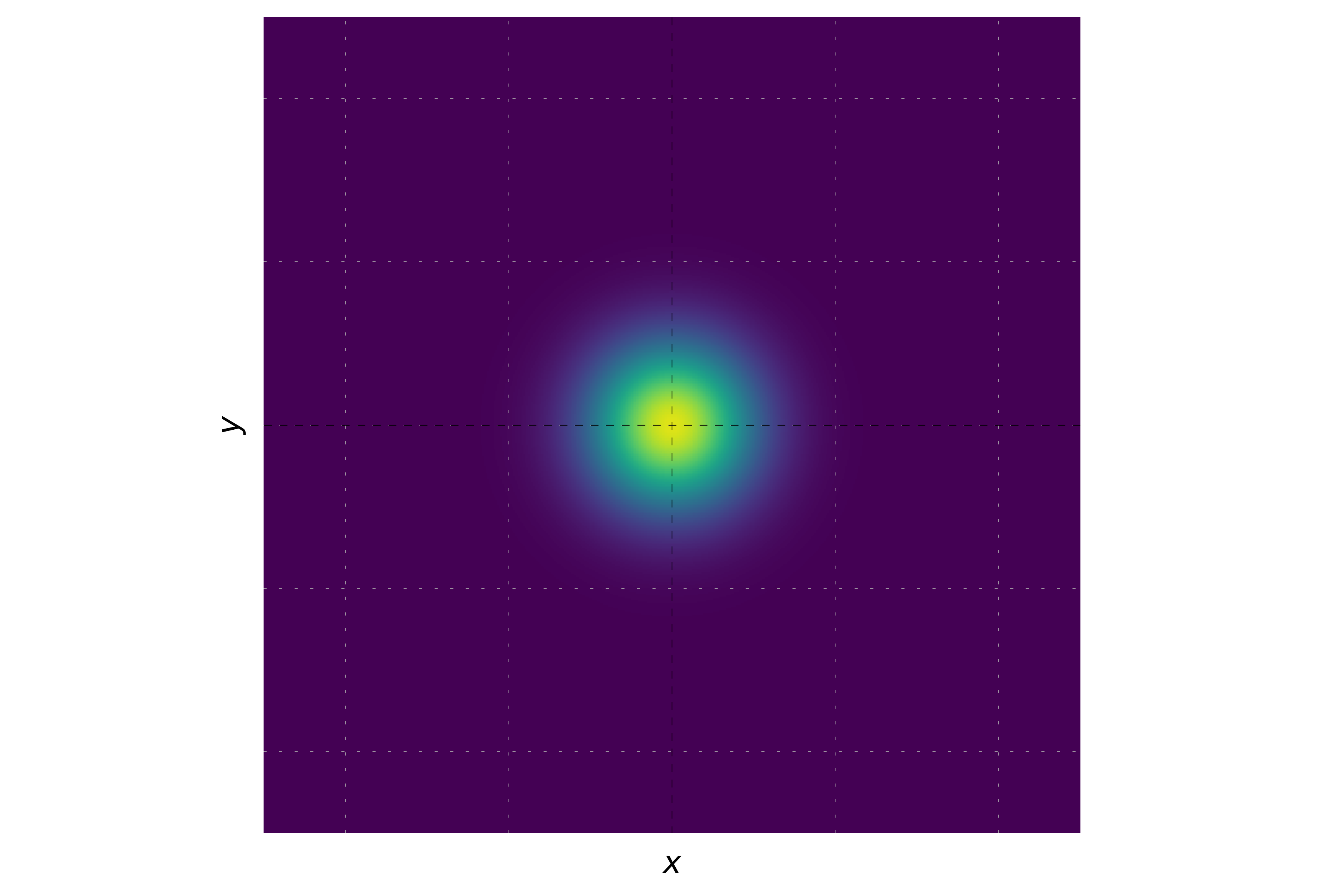
When the momentum is zero, the phase of the wavepacket remains constant. This results in a uniform hue across the entire wavepacket. The probability density will be a Gaussian distribution centered at the origin, and the hue will be consistent, reflecting the constant phase.

When the momentum is only in the x direction, the phase of the wavepacket varies along the x-axis but remains constant along the y-axis. This creates a pattern of stripes oriented parallel to the y-axis. Each stripe represents a region of constant phase. The probability density will still show a Gaussian distribution, but the hue will change periodically along the x-axis.

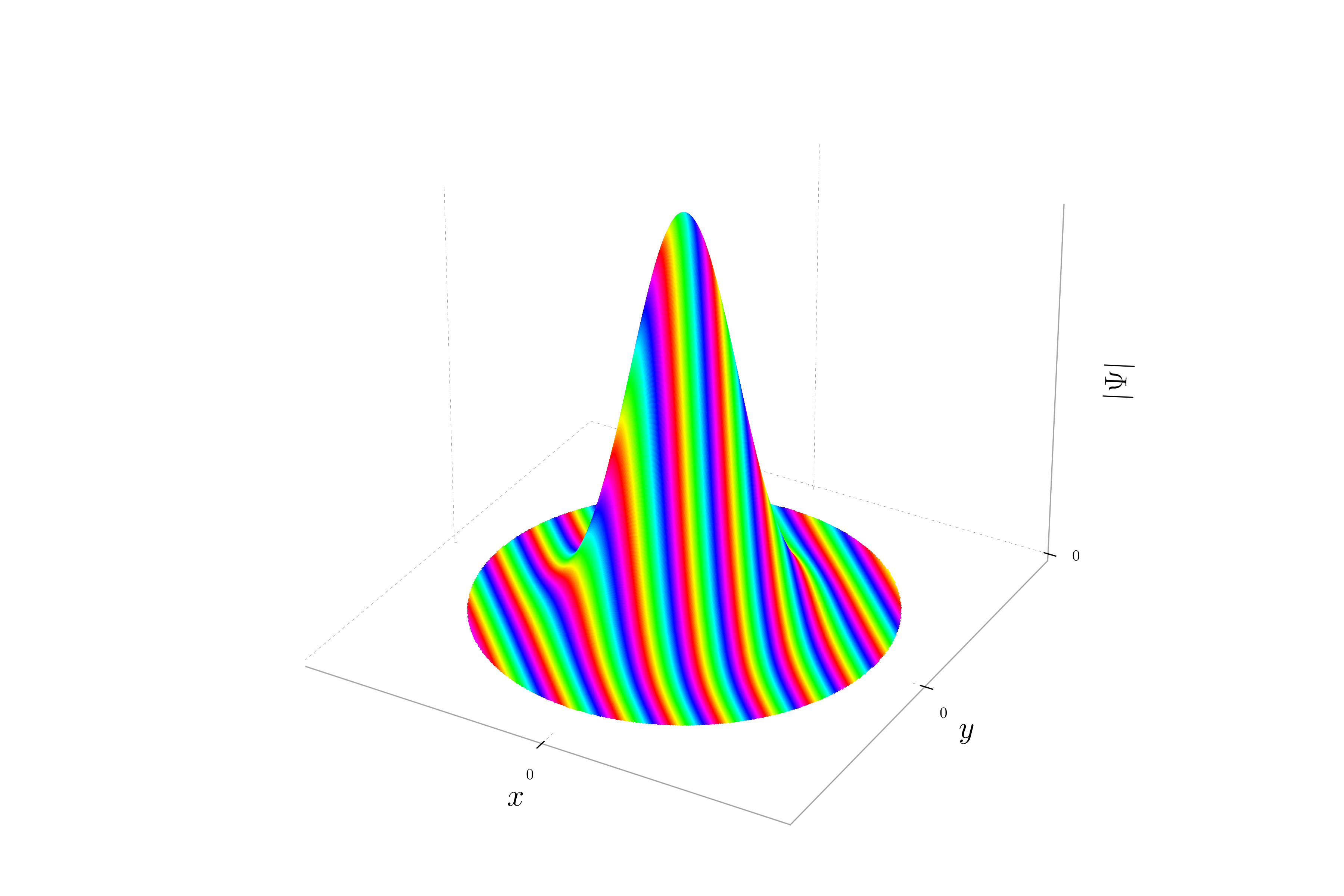
When the momentum is oriented with equal magnitude in both the x and y directions, the phase of the wavepacket varies equally along both axes. This results in stripes oriented at a 45-degree angle to the axes. The probability density remains Gaussian, but the hue will change periodically along a diagonal direction, reflecting the equal contributions of momentum in both x and y directions.

Go to the top of the page