3D Rigid Body Kinetics
Translational Transformation of Inertia Properties
Rotational Transformation of Inertia Properties
Angular momentum
To derive the angular momentum of a rigid body for 3D motion about a point \mathbf{P} using the same conventions, we will follow a similar step-by-step process as the plan rigid body case here.

The angular momentum of a rigid body about a point \mathbf{P} is given as:
\mathbf{L}_P = \int (\mathbf{r} \times \mathbf{v}) \, \mathrm{d}m
where:
- \mathbf{r} is the position vector from point \mathbf{P} to a differential mass element \mathrm{d}m,
- \mathbf{v} is the velocity of the mass element \mathrm{d}m.
For rigid body motion, the velocity \mathbf{v} of each mass element can be described in terms of the velocity of the reference point \mathbf{P} and the angular velocity of the body. Using relative velocity kinematics, the velocity of a mass element at position \mathbf{r} relative to \mathbf{P} is:
\mathbf{v} = \mathbf{v}_P + \boldsymbol{\omega} \times \mathbf{r}
where:
- \mathbf{v}_P is the translational velocity of point \mathbf{P},
- \boldsymbol{\omega} = \omega_x \, \mathbf{i} + \omega_y \, \mathbf{j} + \omega_z \, \mathbf{k} is the angular velocity of the body.
Substitute \mathbf{v} into the expression for \mathbf{L}_P:
\mathbf{L}_P = \int \mathbf{r} \times (\mathbf{v}_P + \boldsymbol{\omega} \times \mathbf{r}) \, \mathrm{d}m
Expand the cross product inside the integral:
\mathbf{L}_P = \int \mathbf{r} \times \mathbf{v}_P \, \mathrm{d}m + \int \mathbf{r} \times (\boldsymbol{\omega} \times \mathbf{r}) \, \mathrm{d}m
The first term is:
\int \mathbf{r} \times \mathbf{v}_P \, \mathrm{d}m
Since \mathbf{v}_P is constant everywhere for the rigid body, it can be factored out of the integral:
\int \mathbf{r} \times \mathbf{v}_P \, \mathrm{d}m = \left( \int \mathbf{r} \, \mathrm{d}m \right) \times \mathbf{v}_P
Define the position vector of the center of mass \mathbf{r}_{C} as:
\mathbf{r}_C = \frac{1}{m} \int \mathbf{r} \, \mathrm{d}m
where m is the total mass of the rigid body. Substituting this back:
\int \mathbf{r} \times \mathbf{v}_P \, \mathrm{d}m = m \, \mathbf{r}_{PC} \times \mathbf{v}_P
where \mathbf{r}_{PC} is the position vector from \mathbf{P} to the center of mass \mathbf{C}.
The second term is:
\int \mathbf{r} \times (\boldsymbol{\omega} \times \mathbf{r}) \, \mathrm{d}m
Using the vector triple product identity:
\mathbf{a} \times (\mathbf{b} \times \mathbf{c}) = (\mathbf{a} \cdot \mathbf{c}) \mathbf{b} - (\mathbf{a} \cdot \mathbf{b}) \mathbf{c}
we expand:
\mathbf{r} \times (\boldsymbol{\omega} \times \mathbf{r}) = (\mathbf{r} \cdot \mathbf{r}) \boldsymbol{\omega} - (\mathbf{r} \cdot \boldsymbol{\omega}) \mathbf{r}
This gives:
\int \mathbf{r} \times (\boldsymbol{\omega} \times \mathbf{r}) \, \mathrm{d}m = \int \big[ (\mathbf{r} \cdot \mathbf{r}) \boldsymbol{\omega} - (\mathbf{r} \cdot \boldsymbol{\omega}) \mathbf{r} \big] \, \mathrm{d}m
Separate the terms:
\int \mathbf{r} \times (\boldsymbol{\omega} \times \mathbf{r}) \, \mathrm{d}m = \boldsymbol{\omega} \int (\mathbf{r} \cdot \mathbf{r}) \, \mathrm{d}m - \int (\mathbf{r} \cdot \boldsymbol{\omega}) \mathbf{r} \, \mathrm{d}m
Expand (\mathbf{r} \cdot \mathbf{r}), which is the square of the magnitude of \mathbf{r}:
\int (\mathbf{r} \cdot \mathbf{r}) \, \mathrm{d}m = \int (x^2 + y^2 + z^2) \, \mathrm{d}m
Expand (\mathbf{r} \cdot \boldsymbol{\omega}):
(\mathbf{r} \cdot \boldsymbol{\omega}) = \omega_x x + \omega_y y + \omega_z z
and \mathbf{r} = x \, \mathbf{i} + y \, \mathbf{j} + z \, \mathbf{k}. Substituting:
\int (\mathbf{r} \cdot \boldsymbol{\omega}) \mathbf{r} \, \mathrm{d}m = \int \big[ (\omega_x x + \omega_y y + \omega_z z)(x \, \mathbf{i} + y \, \mathbf{j} + z \, \mathbf{k}) \big] \, \mathrm{d}m
With the definition of moments and products of inertia:
\begin{aligned} I_{xx} & = \int (y^2 + z^2) \, \mathrm{d}m\\ I_{yy} &= \int (x^2 + z^2) \, \mathrm{d}m \\ I_{zz} & = \int (x^2 + y^2) \, \mathrm{d}m \\ I_{xy} &= -\int xy \, \mathrm{d}m \\ I_{xz} &= -\int xz \, \mathrm{d}m \\ I_{yz} &= -\int yz \, \mathrm{d}m \end{aligned}
The integral can be replaced and the angular momentum can then be written as:
\begin{aligned} \mathbf{L}_P = & m \, \mathbf{r}_{PC} \times \mathbf{v}_P \\ & + \left( I_{xx} \omega_x + I_{xy} \omega_y + I_{xz} \omega_z \right)\mathbf{i} \\ & + \left( I_{xy} \omega_x + I_{yy} \omega_y + I_{yz} \omega_z \right)\mathbf{j} \\ & + \left( I_{xz} \omega_x + I_{yz} \omega_y + I_{zz} \omega_z \right)\mathbf{k} \end{aligned}
Using the moment of inertia tensor, defined as:
\mathbf{I}_P = \begin{bmatrix} I_{xx} & I_{xy} & I_{xz} \\ I_{xy} & I_{yy} & I_{yz} \\ I_{xz} & I_{yz} & I_{zz} \end{bmatrix}
The angular momentum can be written as:
\mathbf{L}_P = m \, \mathbf{r}_{PC} \times \mathbf{v}_P + \mathbf{I}_P \boldsymbol{\omega}
This tensor is symmetric, and it includes information about the mass, shape and geometry of the body.
If \mathbf P is the center of mass, \mathbf{r}_{PC} = 0 the term \mathbf{r}_p \times m \mathbf{v}_p vanishes:
\mathbf L_C = \mathbf{I}_C \boldsymbol{\omega}
If \mathbf P is a point \mathbf A which is fixed in an inertial reference frame (for example it is anchored), \mathbf{V}_{A} = 0 If p has no velocity (\mathbf{v}_p = 0), the term \mathbf{r}_p \times m \mathbf{v}_p vanishes:
\mathbf L_A = \mathbf{I}_A \boldsymbol{\omega}
Translational transformation of inertia properties
A translational transformation shifts an object by a vector \mathbf{r} without rotation:
\mathbf{x}' = \mathbf{x} + \mathbf{r}
A translational transformation of inertia property involves shifting the reference point of an object’s inertia tensor, without altering its orientation. It is useful because it relates the inertia tensor calculated at the center of mass to any other point, which simplifies dynamics analysis when considering motion about axes that are not through the center of mass and makes it easier to decompose motion analysis into separate translational and rotational components. It allows to use the parallel axis theorem and handle cases with complex motion.
For a rigid body, the parallel axis theorem in three dimensions relates the moment of inertia tensor about any axis to the moment of inertia tensor about a parallel axis through the center of mass.
Consider a rigid body with mass m and a point mass m at position \mathbf r relative to an arbitrary origin \mathbf O. The center of mass is at position \mathbf r_{cm} relative to \mathbf O. Let’s denote \mathbf r' as the position vector from the center of mass to the point mass.
\mathbf r' = \mathbf r - \mathbf r_C
The moment of inertia tensor about \mathbf O is:
I_{ij} = \int \left(r^2\delta_{ij} - r_ir_j\right)\mathrm{d}m
For the center of mass, the moment of inertia tensor is:
I^C_{ij} = \int \left({r'}^2\delta_{ij} - r'_ir'_j\right)\mathrm{d}m
Substituting \mathbf r = \mathbf r' + \mathbf r_{C}:
I_{ij} = \int \left[\left({r'}^2 + r_C^2 + 2\mathbf r' \cdot \mathbf r_C\right)\delta_{ij} - \left(r'_i + r_{C,i}\right)\left(r'_j + r_{C,j}\right)\right] \mathrm{d}m
Expanding and using \int \mathbf r'\mathrm{d}m = 0 (definition of center of mass):
I_{ij} = I^C_{ij} + m\left(r_C^2\delta_{ij} - r_{C,i}r_{C,j}\right)
This is the parallel axis theorem in tensor form. In matrix notation:
\mathbf I = \mathbf I_{C} + m \left[\left\|\mathbf r_{C}\right\|^2\mathbf 1 - \mathbf r_{C}\mathbf r_{C}^T\right]
where \mathbf 1 is the identity matrix and \mathbf r_{C}\mathbf r_{C}^T is the outer product. If \mathbf r_1 = \mathbf r_0 - \mathbf d, and substituting this into the moment of inertia equation proves the theorem through direct calculation.
In Cartesian coordinates, if \mathbf d = (d_x, d_y, d_z) is the displacement vector from the center of mass to the point where we want to calculate the moment of inertia:
\mathbf I = \begin{bmatrix} I_{xx} & I_{xy} & I_{xz} \\ I_{xy} & I_{yy} & I_{yz} \\ I_{xz} & I_{yz} & I_{zz} \end{bmatrix} = \begin{bmatrix} I_{xx}^C & I_{xy}^C & I_{xz}^C \\ I_{xy}^C & I_{yy}^C & I_{yz}^C \\ I_{xz}^C & I_{yz}^C & I_{zz}^C \end{bmatrix} + m \begin{bmatrix} d_y^2+d_z^2 & -d_xd_y & -d_xd_z \\ -d_xd_y & d_x^2+d_z^2 & -d_yd_z \\ -d_xd_z & -d_yd_z & d_x^2+d_y^2 \end{bmatrix}
As example, it is possible to compute the moment of inertia of a cuboid with respect to the top left corner,\mathbf d = (\frac{h}{2}, \frac{w}{2}, -\frac{d}{2}).
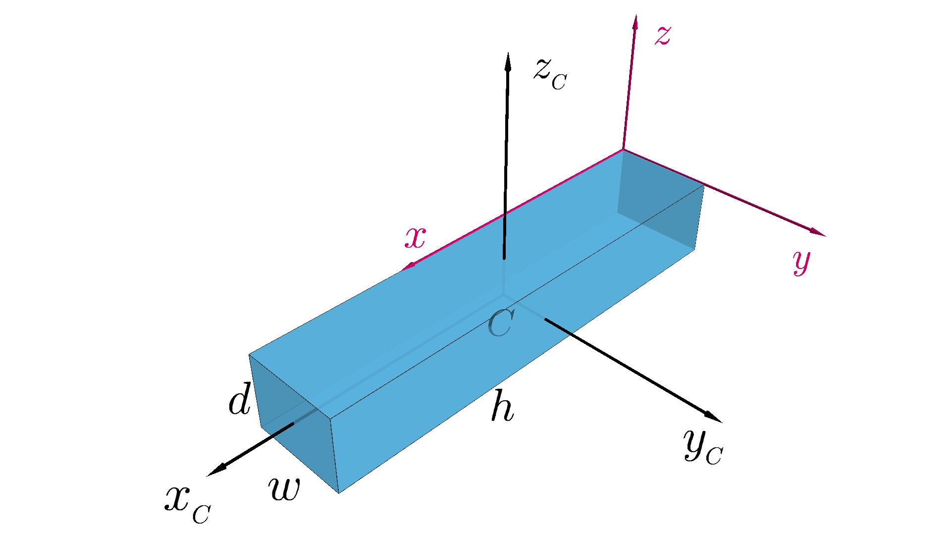
Applying this theorem and using the matrix of inertia here:
\begin{aligned} \mathbf I & = \begin{bmatrix} I_{xx}^C & I_{xy}^C & I_{xz}^C \\ I_{xy}^C & I_{yy}^C & I_{yz}^C \\ I_{xz}^C & I_{yz}^C & I_{zz}^C \end{bmatrix} + m \begin{bmatrix} d_y^2+d_z^2 & -d_xd_y & -d_xd_z \\ -d_xd_y & d_x^2+d_z^2 & -d_yd_z \\ -d_xd_z & -d_yd_z & d_x^2+d_y^2 \end{bmatrix} \\ & = \begin{bmatrix} \frac{m}{12}(w^2 + d^2) & 0 & 0 \\ 0 & \frac{m}{12}(h^2 + d^2) & 0 \\ 0 & 0 & \frac{m}{12}(h^2 + w^2) \end{bmatrix} + m \begin{bmatrix} \frac{d^2 + w^2}{4} & -\frac{h w}{4} & \frac{h d}{4} \\ -\frac{h w}{4} & \frac{h^2 + d^2}{4} & \frac{w d}{4} \\ \frac{h d}{4} & \frac{w d}{4} & \frac{h^2 + w^2}{4} \end{bmatrix} \\ & =\begin{bmatrix} \frac{m}{3}(w^2 + d^2) & -\frac{m h w}{4} & \frac{m h d}{4} \\ -\frac{m h w}{4} & \frac{m}{3}(h^2 + d^2) & \frac{m w d}{4} \\ \frac{m h d}{4} & \frac{m w d}{4} & \frac{m}{3}(h^2 + w^2) \end{bmatrix} \end{aligned}
The matrix of inertia is still symmetric, but is it no longer diagonal, products of inertia are now present because the body doesn’t have any axis of symmetric with respect to the new reference point.
For a numerical example, let’s consider a box with these data:
\begin{aligned} & m = 100 \, \text{kg} \\ & a = 10 \, \text{m} \\ & b = 6 \, \text{m} \\ & d = 4 \, \text{m} \end{aligned}
The matrix of inertia is:
\begin{aligned} \mathbf I = & \begin{bmatrix} \frac{100}{3}(6^2 + 4^2) & -\frac{100 \cdot 10 \cdot 6}{4} & \frac{100 \cdot 10 \cdot 4}{4} \\ -\frac{100 \cdot 10 \cdot 6}{4} & \frac{100}{3}(10^2 + 4^2) & \frac{100 \cdot 6 \cdot 4}{4} \\ \frac{100 \cdot 10 \cdot 4}{4} & \frac{100 \cdot 6 \cdot 4}{4} & \frac{100}{3}(10^2 + 6^2) \end{bmatrix} \\ & = \begin{bmatrix} 1733 & -1500 & 1000 \\ -1500 & 3867 & 600 \\ 1000 & 600 & 4533 \end{bmatrix} \mathrm{kg \cdot m^2} \end{aligned}
Rotational transformation of inertia properties
A rotational transformation of the inertia tensor involves changing its representation from one coordinate system to another due to a rotation.
It is possible to derive the formula based on the theory of rotation transformation matrices here.
Let \mathbf v be an arbitrary vector. The transformation of its components from frame 1 to frame 2 is achieved through a rotation matrix \mathbf T such that:
\mathbf v_2 = \mathbf T \mathbf v_1
where \mathbf v_1 and \mathbf v_2 represent the vector \mathbf v expressed in frames 1 and 2, respectively.
The angular momentum \mathbf L is defined as
\mathbf L = \mathbf I \boldsymbol\omega
where \mathbf I is the inertia matrix and \boldsymbol\omega is the angular velocity vector.
Applying the transformation to the angular momentum in the two frames, we get:
\begin{aligned} & \mathbf L_1 = \mathbf I_1 \boldsymbol\omega_1 \\ & \mathbf L_2 = \mathbf I_2 \boldsymbol\omega_2 \end{aligned}
Since \mathbf L is a vector it also transforms as:
\mathbf L_2 = \mathbf T \mathbf L_1
also since \boldsymbol\omega is a vector, we have
\boldsymbol\omega_2 = \mathbf T \boldsymbol\omega_1
Substituting the angular momentum equation into the transformation equation, we have:
\mathbf I_2 \boldsymbol\omega_2 = \mathbf T \mathbf I_1 \boldsymbol\omega_1
Using the transformation of the angular velocity, we get:
\mathbf I_2 \boldsymbol \omega_2 = \mathbf T \mathbf I_1 \mathbf T ^{-1} \boldsymbol\omega_2
Since the two sides must be equal:
\mathbf I_2 = \mathbf T \mathbf I_1 \mathbf T^{-1}
Since rotation matrices are orthonormal matrices, their inverse is equal to their transpose:
\mathbf I_2 = \mathbf T \mathbf I_1 \mathbf T^T
This equation allows us to compute the inertia matrix in frame 2 given the inertia matrix in frame 1 and the rotation matrix.
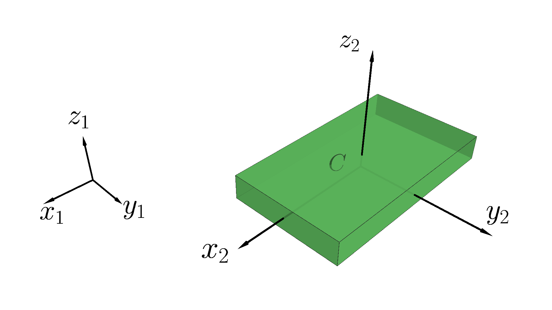
It is possible to continue on the previous example and compute the matrix of inertia of the prism with respect to a rotated axes, for which the \mathbf x_2 axis go through the diagonal, and the \mathbf y_2 axis lies on the plane of the upper face.
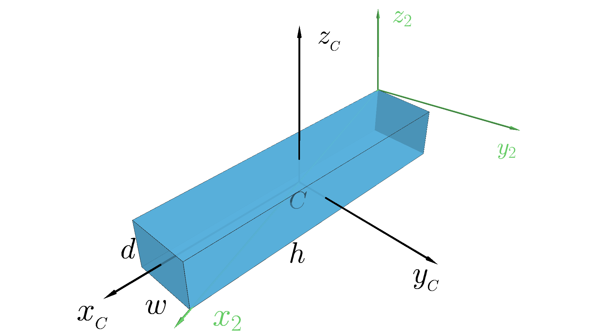
To determine the matrix of inertia, it is necessary to derive the rotation matrix.
As a vector \mathbf v is given (the diagonal) the axis \mathbf x_2 is equal to its normalized version:
\begin{aligned} \mathbf{x}_2 & = \frac{\mathbf v}{\|\mathbf v\|} \\ & = \frac{10 \, \mathbf i + 6 \, \mathbf j - 4 \, \mathbf k}{\sqrt{10^2 + 6^2 +(-4)^2}} \\ & = 0.811 \, \mathbf i + 0.487 \, \mathbf j -0.324 \, \mathbf k \end{aligned}
To find \mathbf y_2 in the x-y plane, it is necessary to determine a vector \mathbf u = (a, b, 0) orthogonal to \mathbf x_2:
\mathbf x_2 \cdot \mathbf u = 0
Any solution works; for simplicity u = -x_{2y}, \, b = x_{2x}, and the normalize it:
\begin{aligned} \mathbf{y}_2 & = \frac{\mathbf u}{\|\mathbf u\|} \\ & = \frac{-0.487 \, \mathbf i + 0.811 \, \mathbf j}{\sqrt{(-0.487)^2 + (0.811)^2}} \\ & = 0.514 \, \mathbf i + 0.857 \, \mathbf j \end{aligned}
Finally \mathbf z_2 is computed as:
\begin{aligned} \mathbf{z}_2 & = \mathbf{x}_2 \times \mathbf{y}_2 \\ & = 0.278 \, \mathbf i + 0.167 \, \mathbf j + 0.946 \, \mathbf k \end{aligned}
The rotation matrix \mathbf{T} maps vectors from the new basis (\mathbf{x}_2, \mathbf{y}_2, \mathbf{z}_2) to the original basis (\mathbf{x}, \mathbf{y}, \mathbf{z}).
To compute it, we start by expressing both the original and new bases as matrices. The original basis is represented as \mathbf{B} = \begin{bmatrix} \mathbf{x} & \mathbf{y} & \mathbf{z} \end{bmatrix}, while the new basis is represented as \mathbf{B_2} = \begin{bmatrix} \mathbf{x}_2 & \mathbf{y}_2 & \mathbf{z}_2 \end{bmatrix}.
The relation between the two bases is \mathbf{B} = \mathbf{T} \cdot \mathbf{B}_2. To solve for \mathbf{T}, multiply through by \mathbf{B}^{-1}_2, giving:
\mathbf{T} = \mathbf{B} \cdot \mathbf{B}^{-1}_2
In the particular case where the original basis vectors in the standard coordinate system are simply \mathbf{i} = (1, 0, 0), \mathbf{j} = (0, 1, 0), and \mathbf{k} = (0, 0, 1), \mathbf B^{-1} = \mathbf 1 and \mathbf B^{-1}_2 = \mathbf B_2^T and the rotation matrix simplifies to:
\begin{aligned} \mathbf{T} &= \mathbf{B}_2^T = \begin{bmatrix} \mathbf{x}_2 & \mathbf{y}_2 & \mathbf{z}_2 \end{bmatrix}^T \\ &= \begin{bmatrix} 0.811 & -0.514 & 0.278 \\ 0.487 & 0.857 & 0.167 \\ -0.324 & 0. & 0.946 \end{bmatrix}^T \\ & = \begin{bmatrix} 0.811 & 0.487 & -0.324 \\ -0.514 & 0.857 & 0. \\ 0.278 & 0.167 & 0.946 \end{bmatrix} \end{aligned}
The new matrix of inertia can now be computed:
\begin{aligned} \mathbf I_2 = & \mathbf T \, \mathbf I \, \mathbf T^T \\ = & \begin{bmatrix} 0.811 & 0.487 & -0.324 \\ -0.514 & 0.857 & 0. \\ 0.278 & 0.167 & 0.946 \end{bmatrix} \begin{bmatrix} 1733 & -1500 & 1000 \\ -1500 & 3867 & 600 \\ 1000 & 600 & 4533 \end{bmatrix} \\ & \begin{bmatrix} 0.811 & -0.514 & 0.278 \\ 0.487 & 0.857 & 0.167 \\ -0.324 & 0. & 0.946 \end{bmatrix} \mathrm{kg \cdot m^2} \\ = & \begin{bmatrix} 633 & 223 & -171 \\ 223 & 4625 & 76 \\ -171 & 76 & 4874 \end{bmatrix} \mathrm{kg \cdot m^2} \end{aligned}
Principal axes
In the general case, the inertia matrix has nine components:
\mathbf I = \begin{bmatrix} I_{xx} & I_{xy} & I_{xz} \\ I_{xy} & I_{yy} & I_{yz} \\ I_{xz} & I_{yz} & I_{zz} \end{bmatrix}
However, for a specific coordinate orientation, the off-diagonal terms (I_{xy}, I_{xz}, I_{yz}) can become zero. When this occurs, the inertia matrix simplifies to a diagonal matrix:
\mathbf I' = \begin{bmatrix} I_1 & 0 & 0 \\ 0 & I_2 & 0 \\ 0 & 0 & I_3 \end{bmatrix}
The axes corresponding to this special coordinate orientation (x_1, y_1, z_1) the principal axes of the body at the chosen point. These axes represent a unique set of axes for which the rotational inertia is particularly straightforward to analyze. The diagonal elements of the inertia matrix in this principal axis frame are the principal moments of inertia.
Considering the angular momentum equation for a rigid body about its center of mass C:
\mathbf{L}_C = \begin{bmatrix} I_{xx}^C & I_{xy}^C & I_{xz}^C \\ I_{xy}^C & I_{yy}^C & I_{yz}^C \\ I_{xz}^C & I_{yz}^C & I_{zz}^C \end{bmatrix} \begin{bmatrix} \omega_x \\ \omega_y \\ \omega_z \end{bmatrix}
Considering a case where the x-axis is aligned with the angular velocity:
\boldsymbol \omega = \omega \mathbf{i}
where \mathbf{i} is the unit vector along the x-axis.
In this case, the angular momentum becomes:
\mathbf{L}_C = I_{xx}^C \omega \mathbf{i} + I_{xy}^C \omega \mathbf{j} + I_{xz}^C \omega \mathbf{k}
\mathbf{L}_C is parallel to \boldsymbol{\omega} if and only if I_{xy}^C=I_{xz}^C=0. This is the defining condition for the x-axis to be a principal axis.
A principal axis is a special axis about which a rigid body can spin without requiring any external torques (or moments) to maintain that rotation.
The inertia tensor in an arbitrary coordinate system is represented by a symmetric 3 \times 3 matrix:
\mathbf I = \begin{bmatrix} I_{xx} & I_{xy} & I_{xz} \\ I_{xy} & I_{yy} & I_{yz} \\ I_{xz} & I_{yz} & I_{zz} \end{bmatrix}
Under a rotation transformation \mathbf R, the inertia tensor transforms as:
\mathbf I' = \mathbf R^T \mathbf I \mathbf R
The principal axes are those directions where the transformed inertia tensor becomes diagonal. In these directions, when the inertia tensor operates on a vector, it produces a vector parallel to the original:
\mathbf I \mathbf e'_i = \lambda_i \mathbf e'_i
This leads to an eigenvalue equation:
\mathbf I \mathbf v = \lambda \mathbf v
Rearranging:
(\mathbf I - \lambda \mathbf 1)\mathbf v = 0
where \mathbf 1 is the 3 \times 3 identity matrix. For non-trivial solutions:
\det(\mathbf I - \lambda \mathbf 1) = 0
Expanding it:
\begin{vmatrix} I_{xx}-\lambda & I_{xy} & I_{xz} \\ I_{xy} & I_{yy}-\lambda & I_{yz} \\ I_{xz} & I_{yz} & I_{zz}-\lambda \end{vmatrix} = 0
The characteristic polynomial for this equation is:
-\lambda^3 + (I_{xx}+I_{yy}+I_{zz})\lambda^2 - (I_{xx}I_{yy}+I_{yy}I_{zz}+I_{xx}I_{zz}-I_{xy}^2-I_{yz}^2-I_{xz}^2)\lambda + \det(\mathbf I) = 0
The eigenvalues (the solutions of this cubic equation) are the principal moments of inertia I_1, I_2, I_3. For each eigenvalue I_k, the corresponding eigenvector \mathbf v_k is found by solving:
(\mathbf I - I_k \mathbf 1)\mathbf v_k = 0
These eigenvectors form the columns of the rotation matrix \mathbf R that transforms from the original coordinate system (x,y,z) to the principal axes (x_1,x_2,x_3):
\mathbf R = [\mathbf v_1 \; \mathbf v_2 \; \mathbf v_3]
resulting in the diagonalized inertia tensor:
\mathbf I' = \begin{bmatrix} I_1 & 0 & 0 \\ 0 & I_2 & 0 \\ 0 & 0 & I_3 \end{bmatrix}
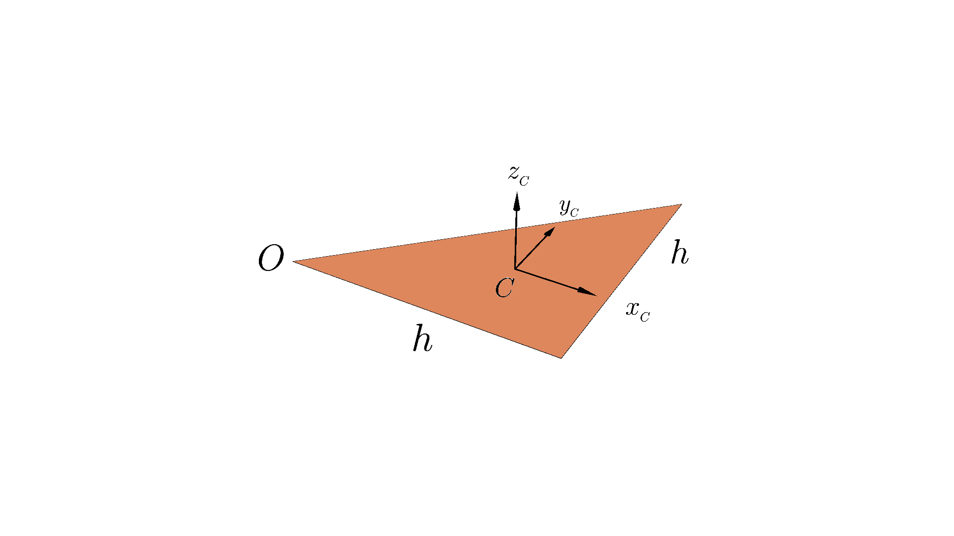
Sample problem
We consider a triangle rectangle with uniform density \rho, where the triangle base is in the xy-plane with vertices at (0, 0, 0), (h,0,0), and (h, h, 0). The element has a smaller vertical component so it is considered negligible.
The tensor of inertia is computed here:
\mathbf{I} = \begin{bmatrix} I_{xx} & I_{xy} & I_{xz} \\ I_{xy} & I_{yy} & I_{yz} \\ I_{xz} & I_{yz} & I_{zz} \end{bmatrix} = \frac{mh^2}{36} \begin{bmatrix} 2 & -1 & 0 \\ -1 & 2 & 0 \\ 0 & 0 & 4 \end{bmatrix}
Principal axes
Now it is possible to work the eigenvalue problem for the matrix:
\mathbf M = \begin{bmatrix} 2 & -1 & 0 \\ -1 & 2 & 0 \\ 0 & 0 & 4 \end{bmatrix}
Eigenvalues
Writing the equation:
\mathbf M - \lambda \mathbf 1 = \begin{bmatrix} 2-\lambda & -1 & 0 \\ -1 & 2-\lambda & 0 \\ 0 & 0 & 4-\lambda \end{bmatrix}
The characteristic polynomial is given by the determinant of \mathbf M - \lambda \mathbf 1:
p(\lambda) = \det(\mathbf M - \lambda \mathbf 1)
We can compute the determinant by cofactor expansion along the third row:
p(\lambda) = 0 \cdot C_{31} + 0 \cdot C_{32} + (4-\lambda) \cdot C_{33} = (4-\lambda) C_{33}
where C_{33} is the (3,3)-cofactor, given by:
\begin{aligned} C_{33} & = (-1)^{3+3} \det \begin{bmatrix} 2-\lambda & -1 \\ -1 & 2-\lambda \end{bmatrix} = \det \begin{bmatrix} 2-\lambda & -1 \\ -1 & 2-\lambda \end{bmatrix} \\ & = (2-\lambda)(2-\lambda) - (-1)(-1) = (2-\lambda)^2 - 1 = 4 - 4\lambda + \lambda^2 - 1 = \lambda^2 - 4\lambda + 3 \end{aligned}
The characteristic polynomial is:
p(\lambda) = (4-\lambda) (\lambda^2 - 4\lambda + 3)
We can factor the quadratic term:
\lambda^2 - 4\lambda + 3 = (\lambda - 1) (\lambda - 3)
So the characteristic polynomial is:
p(\lambda) = (4-\lambda) (\lambda - 1) (\lambda - 3)
To find the eigenvalues, we set p(\lambda) = 0:
(4-\lambda) (\lambda - 1) (\lambda - 3) = 0
The eigenvalues are the roots of this polynomial, which are:
\lambda_1 = 1, \quad \lambda_2 = 3, \quad \lambda_3 = 4
The eigenvalues are 1, 3, 4.
Eigenvectors
To compute the eigenvector corresponding to the first eigenvalue \lambda_1 = 1, we need to solve the equation (\mathbf M - \lambda_1 \mathbf 1) \mathbf v_1 = \mathbf 0. For \lambda_1 = 1, we have:
\mathbf M - \mathbf 1 = \begin{bmatrix} 2-1 & -1 & 0 \\ -1 & 2-1 & 0 \\ 0 & 0 & 4-1 \end{bmatrix} = \begin{bmatrix} 1 & -1 & 0 \\ -1 & 1 & 0 \\ 0 & 0 & 3 \end{bmatrix} = \begin{bmatrix} 0 \\ 0 \\ 0 \end{bmatrix}
This gives us the following system of equations:
\begin{aligned} & x - y = 0 \\ & -x + y = 0 \\ & 3z = 0 \end{aligned}
From the first equation, we get x = y. The second equation is equivalent to the first one. From the third equation, we get z = 0. So the eigenvector \mathbf v_1 can be written as:
\mathbf v_1 = \begin{bmatrix} x \\ y \\ z \end{bmatrix} = \begin{bmatrix} x \\ x \\ 0 \end{bmatrix} = x \begin{bmatrix} 1 \\ 1 \\ 0 \end{bmatrix}
We can choose x=1 to get a particular eigenvector \mathbf v_1 = \begin{bmatrix} 1 \\ 1 \\ 0 \end{bmatrix}.
To normalize \mathbf v_1, we need to divide it by its magnitude \|\mathbf v_1\|:
\|\mathbf v_1\| = \sqrt{1^2 + 1^2 + 0^2} = \sqrt{1 + 1 + 0} = \sqrt{2}
The normalized eigenvector \mathbf u_1 is:
\mathbf u_1 = \frac{\mathbf v_1}{\|\mathbf v_1\|} = \frac{1}{\sqrt{2}} \begin{bmatrix} 1 \\ 1 \\ 0 \end{bmatrix} = \begin{bmatrix} 1/\sqrt{2} \\ 1/\sqrt{2} \\ 0 \end{bmatrix}
To compute the eigenvector corresponding to the second eigenvalue \lambda_2 = 3, we need to solve the equation (\mathbf M - \lambda_2 \mathbf 1) \mathbf v_2 = \mathbf 0. For \lambda_2 = 3, we have:
\mathbf M - 3 \mathbf I = \begin{bmatrix} 2-3 & -1 & 0 \\ -1 & 2-3 & 0 \\ 0 & 0 & 4-3 \end{bmatrix} = \begin{bmatrix} -1 & -1 & 0 \\ -1 & -1 & 0 \\ 0 & 0 & 1 \end{bmatrix} = \begin{bmatrix} 0 \\ 0 \\ 0 \end{bmatrix}
This gives us the following system of equations:
\begin{aligned} & -x - y = 0 \\ & -x - y = 0 \\ &z = 0 \end{aligned}
From the first equation, we get y = -x. The third equation gives z = 0. Let x = -1, then y = 1 and z = 0. So, an eigenvector is \mathbf v_2 = \begin{bmatrix} -1 \\ 1 \\ 0 \end{bmatrix}. To normalize \mathbf v_2, we calculate its norm:
\|\mathbf v_2\| = \sqrt{(-1)^2 + 1^2 + 0^2} = \sqrt{1 + 1 + 0} = \sqrt{2}
The normalized eigenvector \mathbf u_2 is:
\mathbf u_2 = \frac{\mathbf v_2}{\|\mathbf v_2\|} = \frac{1}{\sqrt{2}} \begin{bmatrix} -1 \\ 1 \\ 0 \end{bmatrix} = \begin{bmatrix} -1/\sqrt{2} \\ 1/\sqrt{2} \\ 0 \end{bmatrix}
To compute the eigenvector corresponding to the third eigenvalue \lambda_3 = 4, we need to solve the equation (\mathbf M - \lambda_3 \mathbf I) \mathbf v_3 = \mathbf 0. For \lambda_3 = 4, we have:
\mathbf M - 4 \mathbf I = \begin{bmatrix} 2-4 & -1 & 0 \\ -1 & 2-4 & 0 \\ 0 & 0 & 4-4 \end{bmatrix} = \begin{bmatrix} -2 & -1 & 0 \\ -1 & -2 & 0 \\ 0 & 0 & 0 \end{bmatrix} = \begin{bmatrix} 0 \\ 0 \\ 0 \end{bmatrix}
This gives us the following system of equations:
\begin{aligned} & -2x - y = 0 \\ & -x - 2y = 0 \\ & 0 = 0 \end{aligned}
From the first equation, we get y = -2x. Substituting this into the second equation:
\begin{aligned} & -x - 2(-2x) = 0 \\ & -x + 4x = 0 \\ & 3x = 0 \end{aligned}
So x = 0. Then y = -2x = -2(0) = 0. The variable z is free. We can choose z = 1. So the eigenvector is \mathbf v_3 = \begin{bmatrix} 0 \\ 0 \\ 1 \end{bmatrix}. To normalize \mathbf v_3, we calculate its norm:
\|\mathbf v_3\| = \sqrt{0^2 + 0^2 + 1^2} = \sqrt{1} = 1
The normalized eigenvector \mathbf u_3 is:
\mathbf u_3 = \frac{\mathbf v_3}{\|\mathbf v_3\|} = \frac{1}{1} \begin{bmatrix} 0 \\ 0 \\ 1 \end{bmatrix} = \begin{bmatrix} 0 \\ 0 \\ 1 \end{bmatrix}
Diagonalization
The matrix \mathbf M can be diagonalized as \mathbf M = \mathbf P \mathbf D \mathbf P^{-1}, where \mathbf D is a diagonal matrix with the eigenvalues on the diagonal, and \mathbf P is a matrix whose columns are the corresponding eigenvectors.
We found the eigenvalues are \lambda_1 = 1, \lambda_2 = 3, \lambda_3 = 4, and the corresponding normalized eigenvectors are:
\mathbf u_1 = \begin{bmatrix} 1/\sqrt{2} \\ 1/\sqrt{2} \\ 0 \end{bmatrix}, \quad \mathbf u_2 = \begin{bmatrix} -1/\sqrt{2} \\ 1/\sqrt{2} \\ 0 \end{bmatrix}, \quad \mathbf u_3 = \begin{bmatrix} 0 \\ 0 \\ 1 \end{bmatrix}
We can form the matrices \mathbf P and \mathbf D as:
\begin{aligned} \mathbf P & = \begin{bmatrix} 1/\sqrt{2} & -1/\sqrt{2} & 0 \\ 1/\sqrt{2} & 1/\sqrt{2} & 0 \\ 0 & 0 & 1 \end{bmatrix} \\ \mathbf D & = \begin{bmatrix} 1 & 0 & 0 \\ 0 & 3 & 0 \\ 0 & 0 & 4 \end{bmatrix} \end{aligned}
Since the eigenvectors are orthonormal, \mathbf P is an orthogonal matrix, and its inverse is its transpose: \mathbf P^{-1} = \mathbf P^T.
\mathbf P^{-1} = \mathbf P^T = \begin{bmatrix} 1/\sqrt{2} & 1/\sqrt{2} & 0 \\ -1/\sqrt{2} & 1/\sqrt{2} & 0 \\ 0 & 0 & 1 \end{bmatrix}
The diagonalization of \mathbf M is \mathbf M = \mathbf P \mathbf D \mathbf P^{-1} with the matrices \mathbf P, \mathbf D, and \mathbf P^{-1} given above.
To verify that \mathbf M = \mathbf P \mathbf D \mathbf P^{-1}, we need to compute the product \mathbf P \mathbf D \mathbf P^{-1} and check if it is equal to \mathbf M. Since \mathbf P is orthogonal, \mathbf P^{-1} = \mathbf P^T.
First, we compute \mathbf D \mathbf P^T:
\mathbf D \mathbf P^T = \begin{bmatrix} 1 & 0 & 0 \\ 0 & 3 & 0 \\ 0 & 0 & 4 \end{bmatrix} \begin{bmatrix} 1/\sqrt{2} & 1/\sqrt{2} & 0 \\ -1/\sqrt{2} & 1/\sqrt{2} & 0 \\ 0 & 0 & 1 \end{bmatrix} = \begin{bmatrix} 1/\sqrt{2} & 1/\sqrt{2} & 0 \\ -3/\sqrt{2} & 3/\sqrt{2} & 0 \\ 0 & 0 & 4 \end{bmatrix}
Then, we compute \mathbf P (\mathbf D \mathbf P^T):
\begin{aligned} \mathbf P \mathbf D \mathbf P^T & = \begin{bmatrix} 1/\sqrt{2} & -1/\sqrt{2} & 0 \\ 1/\sqrt{2} & 1/\sqrt{2} & 0 \\ 0 & 0 & 1 \end{bmatrix} \begin{bmatrix} 1/\sqrt{2} & 1/\sqrt{2} & 0 \\ -3/\sqrt{2} & 3/\sqrt{2} & 0 \\ 0 & 0 & 4 \end{bmatrix} = \\ & = \begin{bmatrix} 1/2 + 3/2 & 1/2 - 3/2 & 0 \\ 1/2 - 3/2 & 1/2 + 3/2 & 0 \\ 0 & 0 & 4 \end{bmatrix} = \begin{bmatrix} 2 & -1 & 0 \\ -1 & 2 & 0 \\ 0 & 0 & 4 \end{bmatrix} = \mathbf M \end{aligned}
the diagonalized inertia tensor is then:
\mathbf I' = \begin{bmatrix} I_1 & 0 & 0 \\ 0 & I_2 & 0 \\ 0 & 0 & I_3 \end{bmatrix} = \frac{mh^2}{36} \begin{bmatrix} 1 & 0 & 0 \\ 0 & 3 & 0 \\ 0 & 0 & 2 \end{bmatrix}
It is possible to plot the eigenvectors and compare the axis with the original axes.
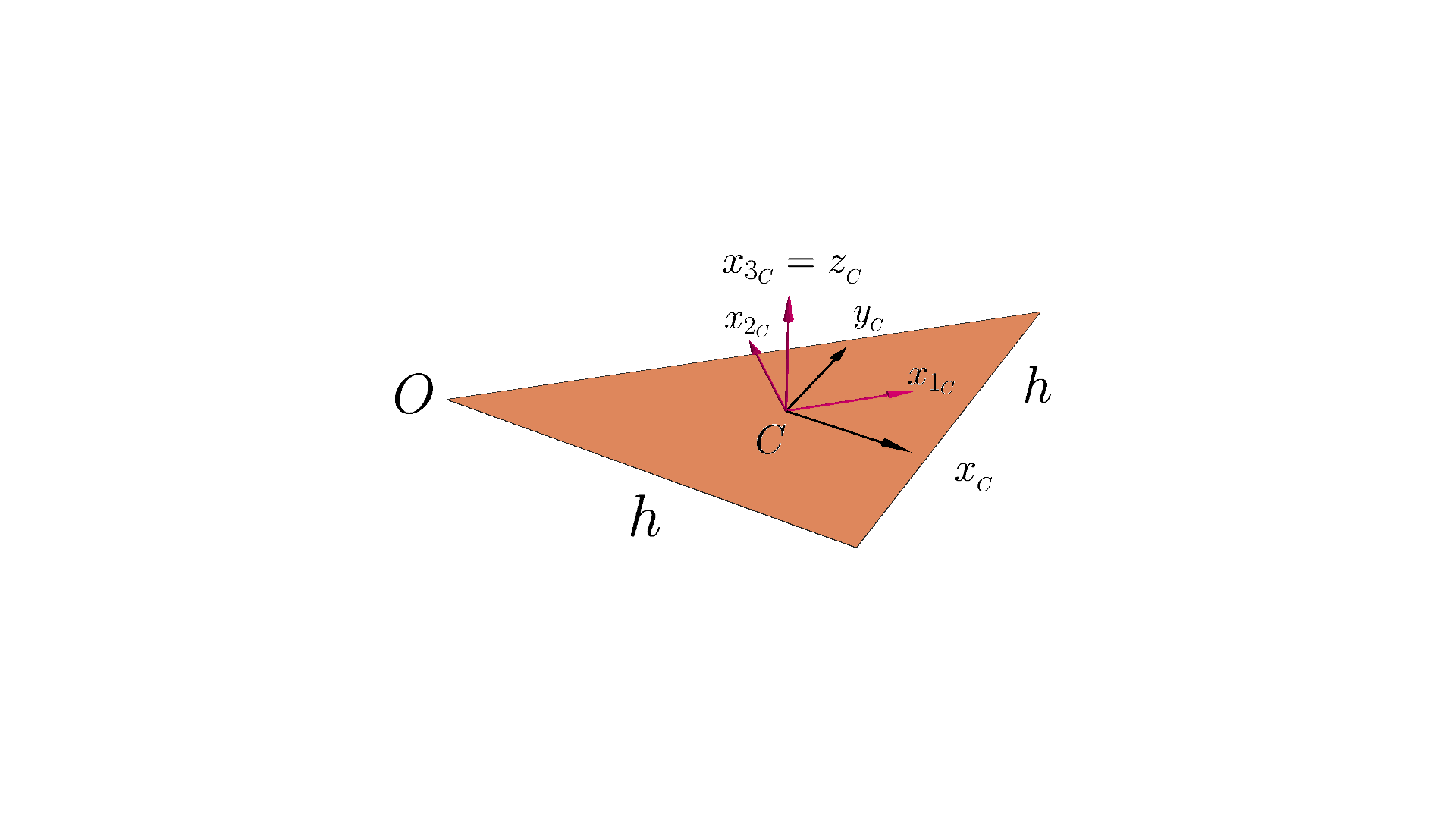
The matrix \mathbf M represents the moment of inertia tensor of a rigid body. The eigenvalues of \mathbf M, which are \lambda_1 = 1, \lambda_2 = 3, \lambda_3 = 4, are the principal moments of inertia along the principal axes of rotation. The corresponding eigenvectors are the directions of these principal axes. The principal moments of inertia indicate the resistance to rotation about the corresponding principal axes.
The first principal axis, corresponding to the smallest eigenvalue \lambda_1 = 1 and eigenvector \mathbf u_1, is the axis around which the object is easiest to rotate, as it has the smallest moment of inertia. A smaller moment of inertia implies that the mass is more concentrated around this axis, requiring less torque to achieve the same angular acceleration. We can call this principal axis the x_1-axis, oriented along \mathbf u_1.
The third principal axis, corresponding to the largest eigenvalue \lambda_3 = 4 and eigenvector \mathbf u_3 = \mathbf k, is the axis around which the object is hardest to rotate, as it has the largest moment of inertia. A larger moment of inertia indicates that the mass is distributed further away from this axis, making it more resistant to rotational motion. This principal axis, which coincides with the z-axis, can be named the x_3-axis.
The second principal axis, with eigenvalue \lambda_2 = 3 and eigenvector \mathbf u_2, has an intermediate moment of inertia value, meaning the resistance to rotation around this axis is between the easiest and hardest cases. We can refer to this principal axis as the x_2-axis.
Equations of motion
Let’s start with a recap the Euler equations are essential. They describe how torques influence a body’s angular momentum.
The fundamental form of Euler’s second law states that the sum of the external moments (torques) about a fixed point O is equal to the rate of change of angular momentum about that point:
\sum \mathbf{M}_O = \frac{\mathrm{d}\mathbf{L}_O}{\mathrm{d}t}
A particularly useful case is when we consider the mass center (C) of the rigid body. Euler’s second law simplifies to:
\sum \mathbf{M}_C = \frac{\mathrm{d}\mathbf{L}_C}{\mathrm{d}t}
If we pick any arbitrary point P in the body, we need to account for the motion of the mass center relative to P:
\sum \mathbf{M}_P = \frac{\mathrm{d}\mathbf{L}_C}{\mathrm{d}t} + \mathbf{r}_{PC} \times m\mathbf{a}_C
where \mathbf{r}_{PC} is the position vector from point P to the mass center C and \mathbf{a}_C is the acceleration of the mass center C.
Let’s choose a body-fixed reference frame 2 welded into the body with axes \mathbf{i}_2, \mathbf{j}_2, \mathbf{k}_2 such that the moments and products of inertia remain constant over time.

Then to compute the derivative of the angular momentum it is necessary to use the derivative vector formula, taking as vector the angular momentum \mathbf L:
\sum \mathbf{M}_C\big|_1 = \frac{\mathrm{d}\mathbf{L}_C}{\mathrm{d}t}\bigg|_1 = \frac{\mathrm{d}\mathbf{L}_C}{\mathrm{d}t}\bigg|_2 + \boldsymbol{\omega}_{2/1} \times \mathbf L_C The angular momentum is equal to the matrix of inertia times the angular velocity (dropping now the index and just writing \boldsymbol \omega:
\mathbf L_C = \mathbf I_C \boldsymbol \omega = \begin{bmatrix} I_{xx} & I_{xy} & I_{xz} \\ I_{xy} & I_{yy} & I_{yz} \\ I_{xz} & I_{yz} & I_{zz} \end{bmatrix} \begin{bmatrix} \omega_x \\ \omega_y \\ \omega_z \end{bmatrix} In the reference frame 2 the moment of inertia is not changing in time by construction so:
\frac{\mathrm{d}\mathbf{L}_C}{\mathrm{d}t}\bigg|_2 = \mathbf I_C \dot{\boldsymbol {\omega}} = \begin{bmatrix} I_{xx} & I_{xy} & I_{xz} \\ I_{xy} & I_{yy} & I_{yz} \\ I_{xz} & I_{yz} & I_{zz} \end{bmatrix} \begin{bmatrix} \dot \omega_x \\ \dot \omega_y \\ \dot \omega_z \end{bmatrix}
The cross product \boldsymbol{\omega} \times \mathbf L_C is equal to:
\begin{aligned} \boldsymbol{\omega} \times \mathbf L_C & = \begin{bmatrix} (I_{zz} - I_{yy}) \omega_y \omega_z + I_{yz} (\omega_y^2 - \omega_z^2) + I_{xz} \omega_x \omega_y - I_{xy} \omega_x \omega_z \\ (I_{xx} - I_{zz}) \omega_x \omega_z + I_{xz} (\omega_z^2 - \omega_x^2) + I_{xy} \omega_y \omega_z - I_{yz} \omega_x \omega_y \\ (I_{yy} - I_{xx}) \omega_x \omega_y + I_{xy} (\omega_x^2 - \omega_y^2) + I_{yz} \omega_x \omega_z - I_{xz} \omega_y \omega_z \end{bmatrix} \end{aligned}
Summing together:
\begin{aligned} \sum M_C = & \left(I_{xx}^C \dot{\omega}_x + I_{xy}^C \dot{\omega}_y + I_{xz}^C \dot{\omega}_z \right) \mathbf i \\ & + \left(I_{yx}^C \dot{\omega}_x + I_{yy}^C \dot{\omega}_y + I_{yz}^C \dot{\omega}_z\right) \mathbf j \\ & + \left(I_{zx}^C \dot{\omega}_x + I_{zy}^C \dot{\omega}_y + I_{zz}^C \dot{\omega}_z\right) \mathbf k \\ & + \left[\left(I_{zz}^C - I_{yy}^C\right)\omega_y\omega_z + I_{yz}^C \left(\omega_z^2 - \omega_y^2\right) + \omega_x\left(I_{xy}^C - I_{xz}^C\right)\right] \mathbf i \\ & + \left[\left(I_{xx}^C - I_{zz}^C\right)\omega_z\omega_x + I_{xz}^C \left(\omega_x^2 - \omega_z^2\right) + \omega_y\left(I_{yz}^C - I_{xy}^C\right)\right] \mathbf j \\ & + \left[\left(I_{yy}^C - I_{xx}^C\right)\omega_x\omega_y + I_{xy}^C \left(\omega_y^2 - \omega_x^2\right) + \omega_z\left(I_{xz}^C - I_{yz}^C\right)\right] \mathbf k \end{aligned}
If we chose the principal axes, the expression simplify greatly as the product of inertia are zero:
\begin{aligned} \sum \mathbf M_C = & \left[I_{xx}^C \dot{\omega}_x - \left(I_{yy}^C - I_{zz}^C\right) \omega_y \omega_z \right] \mathbf i \\ & + \left[I_{yy}^C \dot{\omega}_y - \left(I_{zz}^C - I_{xx}^C\right) \omega_z \omega_x \right] \mathbf j \\ & + \left[I_{zz}^C \dot{\omega}_z - \left(I_{xx}^C - I_{yy}^C\right) \omega_x \omega_y \right] \mathbf k \end{aligned}
These are 3 equations:
\begin{aligned} \sum M_{C_x} = & I_{xx}^C \dot{\omega}_x - \left(I_{yy}^C - I_{zz}^C\right) \omega_y \omega_z \\ \sum M_{C_y} = & I_{yy}^C \dot{\omega}_y - \left(I_{zz}^C - I_{xx}^C\right) \omega_z \omega_x\\ \sum M_{C_z} = & I_{zz}^C \dot{\omega}_z - \left(I_{xx}^C - I_{yy}^C\right) \omega_x \omega_y \end{aligned}
Similar equations can be written for a fixed pivot point:
\begin{aligned} \sum M_{O_x} = & I_{xx}^O \dot{\omega}_x - \left(I_{yy}^O - I_{zz}^O\right) \omega_y \omega_z \\ \sum M_{O_y} = & I_{yy}^O \dot{\omega}_y - \left(I_{zz}^O - I_{xx}^O\right) \omega_z \omega_x\\ \sum M_{O_z} = & I_{zz}^O \dot{\omega}_z - \left(I_{xx}^O - I_{yy}^O\right) \omega_x \omega_y \end{aligned}
Another case that can be useful for solving problems is to use a reference frame when the angular momentum (or the external moments) can be conveniently expressed, and for some reasons (like symmetries for example) the moments of inertia are not changing in this intermediate frame, and in general this intermediate frame 3 has the origin at the mass center or at a fixed pivot point:
\begin{aligned} \sum \mathbf{M}_C & = \frac{\mathrm{d}\mathbf{L}_C}{\mathrm{d}t}\bigg|_3 = \frac{\mathrm{d}\mathbf{L}_C}{\mathrm{d}t}\bigg|_2 + \boldsymbol{\omega}_{3/2} \times \mathbf L_C \\ \sum \mathbf{M}_O & = \frac{\mathrm{d}\mathbf{L}_O}{\mathrm{d}t}\bigg|_3 = \frac{\mathrm{d}\mathbf{L}_O}{\mathrm{d}t}\bigg|_2 + \boldsymbol{\omega}_{3/2} \times \mathbf L_O \end{aligned}
Sample problem
For this problem it is possible to consider again the landing gear previously analyzed for the kinematics here, and now we will look at the moments acting on the body.
Strictly speaking the aircraft is not into an inertial frame, but for this problem we will consider the acceleration negligible and the frame to be inertial.
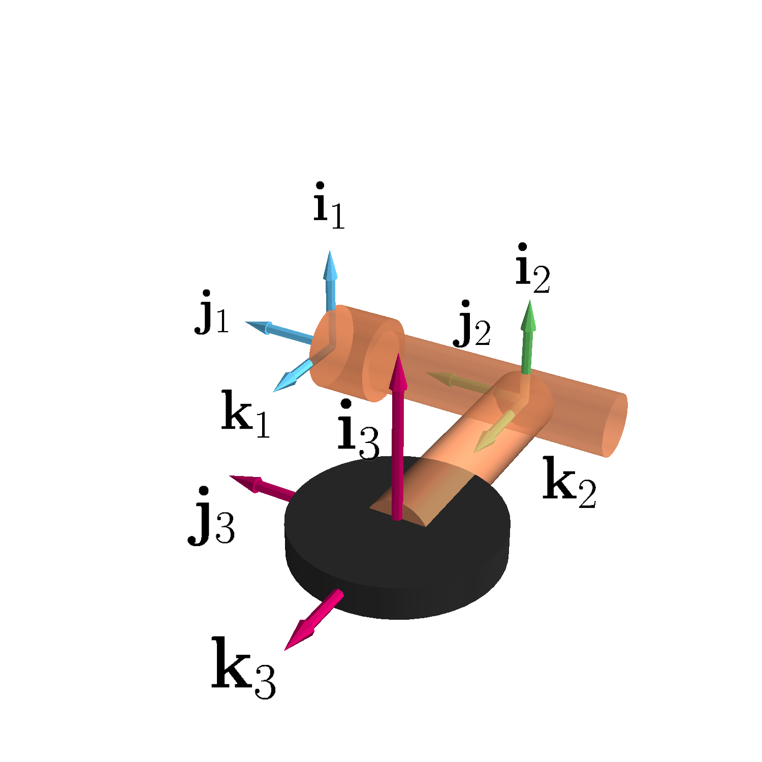
We consider the case where a moment is applied along the y-axis. We will use an intermediate frame in this case (which we call frame 4), and the intermediate frame is fixed on the arm, so it is not rotating with the wheel, so it is not body fixed. The inertial reference frame is still frame 1 as previously:
- the wheel has a diameter r and a thickness h;
- the wheel spins in the \mathbf i_3 direction (\omega_s \mathbf i_3);
- there is a moment \mathbf M_0 applied along the \mathbf j_1 axis which moves with a velocity \omega_y \mathbf j_1.
The objective is to find the rate of change of the wheel \omega_s and the moment reaction ant the point C, which is the point where the wheel is connected to the arm, and there is a bearing there so it is important to know what are the stressed this bearing is subjected to, so it can be properly designed.
The equation that will be used is:
\sum \mathbf{M}_C = \frac{\mathrm{d}\mathbf{L}_C}{\mathrm{d}t}\bigg|_1 = \frac{\mathrm{d}\mathbf{L}_C}{\mathrm{d}t}\bigg|_4 + \boldsymbol{\omega}_{4/1} \times \mathbf L_C
The first step is to find the angular momentum of the wheel with respect to the inertial frame:
\mathbf L_C = \mathbf I_C \boldsymbol \omega_{3/1}
The angular velocity on the inertial frame can be computed with the addition theorem:
\boldsymbol \omega_{3/1} = \boldsymbol \omega_{3/4} + \boldsymbol \omega_{4/1} = \omega_s \mathbf i_1 + \omega_y \mathbf j_1
Because of the symmetry of the wheel, the matrix of inertia in the intermediate frame and on the body frame are the same:
\mathbf I\big|_3 = \mathbf I\big|_4
And for this configuration again due to symmetry these are principal axes. The moment of inertia of a cylinder has been computed here and for this configuration are:
\begin{aligned} & I_{xx_4} = \frac{1}{2}mr^2 = I_1 \\ & I_{yy_4} = I_{zz_4} = \frac{1}{12}m \left( 3r^2 + h^2 \right) = I_2 \end{aligned}
The matrix of inertia is:
\mathbf I \big|_4 =\begin{bmatrix} I_1 & 0 & 0 \\ 0 & I_2 & 0 \\ 0 & 0 & I_2 \end{bmatrix}
Then it is possible to compute the angular momentum:
\begin{aligned} \mathbf L_C & = \mathbf I_C \boldsymbol \omega_{3/1} \\ & = \begin{bmatrix} I_1 & 0 & 0 \\ 0 & I_2 & 0 \\ 0 & 0 & I_2 \end{bmatrix} \begin{bmatrix} \omega_s \\ \omega_y \\ 0 \end{bmatrix} \\ & = I_1 \omega_s \mathbf i_1 + I_2 \omega_y \mathbf j_1 \end{aligned}
Now that the angular momentum it is know, it is possible to apply the formula. The first item to compute is the derivative of the angular momentum in the frame 4 (the frame of the arm).
The inertia frame does not change with time in the frame 4, but the angular velocity can change:
\begin{aligned} \sum \mathbf{M}_C & = \frac{\mathrm{d}\mathbf{L}_C}{\mathrm{d}t}\bigg|_1 = \frac{\mathrm{d}\mathbf{L}_C}{\mathrm{d}t}\bigg|_4 + \boldsymbol{\omega}_{4/1} \times \mathbf L_C \\ & = I_1 \dot \omega_s \mathbf i_1 + I_2 \dot \omega_y \mathbf j_1 + \omega_y \mathbf j_1 \times \mathbf L_C \\ & = I_1 \dot \omega_s \mathbf i_1 + I_2 \dot \omega_y \mathbf j_1 + \omega_y \mathbf j_1 \times \left( I_1\omega_s \mathbf i_1 + I_2 \omega_y \mathbf j_1 \right) \\ & = I_1 \dot \omega_s \mathbf i_1 + I_2 \dot \omega_y \mathbf j_1 - I_2\omega_y\omega_s \mathbf k_1 \end{aligned}
as \boldsymbol{\omega}_{4/1} = \omega_y \mathbf j_1 since the velocity of the arm is simply the velocity retracting into the airplane.
The left hand side is now known, it is necessary to determine now the moments acting on the body. At point C there is a bearing (so that the wheel can spin along \mathbf i_3 = \mathbf i_1 but is not moving in the other two directions):
- there is no acceleration so there is a reaction C_x, C_y, and C_z,
- there is a moment reaction along the axis \mathbf j_3 = \mathbf j_1 M_{C_y} and \mathbf k_3 = \mathbf k_1 and M_{C_z},
- there is the weight mg \mathbf i_3.
The sum of the moments about C are:
\sum \mathbf{M}_C = M_{C_y} \mathbf j_1 + M_{C_z} \mathbf k_1
So the full equation becomes:
M_{C_y} \mathbf j_1 + M_{C_z} \mathbf k_1 = I_1 \dot \omega_s \mathbf i_1 + I_2 \dot \omega_y \mathbf j_1 - I_2\omega_y\omega_s \mathbf k_1
Equating components:
\begin{aligned} & 0 = I_1 \dot \omega_s \\ & M_{C_y} = I_2 \dot \omega_y \\ & M_{C_z} = - I_2\omega_y\omega_s \end{aligned}
Looking at this equations:
- the first one gives that \dot \omega_s = 0 so \omega_s = c constant,
- the second tell that the bigger the moment applies the faster the arm will rotate (which makes physical sense),
- the third one is an interesting discover because while there are velocities only on the \mathbf i_1 and \mathbf j_1 axes, there is a moment around the \mathbf k, which is called a gyroscopic moment.
Sample problem
We can do another example considering a satellite spin stabilization. Let’s approximate the satellite as a cuboid, consider an inertial reference frame 1 and a reference frame 2 welded to the body of the satellite.
For this example, we will be using the equations with respect to the center of mass:
\begin{aligned} \sum M_{C_x} = & I_{xx}^C \dot{\omega}_x - \left(I_{yy}^C - I_{zz}^C\right) \omega_y \omega_z \\ \sum M_{C_y} = & I_{yy}^C \dot{\omega}_y - \left(I_{zz}^C - I_{xx}^C\right) \omega_z \omega_x\\ \sum M_{C_z} = & I_{zz}^C \dot{\omega}_z - \left(I_{xx}^C - I_{yy}^C\right) \omega_x \omega_y \end{aligned}
For free space motion, there are no moments acting on the body M_{C_x} = M_{C_y} = M_{C_z} =0:
\begin{aligned} & I_{xx}^C \dot{\omega}_x - \left(I_{yy}^C - I_{zz}^C\right) \omega_y \omega_z = 0\\ & I_{yy}^C \dot{\omega}_y - \left(I_{zz}^C - I_{xx}^C\right) \omega_z \omega_x = 0\\ & I_{zz}^C \dot{\omega}_z - \left(I_{xx}^C - I_{yy}^C\right) \omega_x \omega_y = 0 \end{aligned}
Furthermore, we assume steady motion, with a constant stabilization about the z-axis (e.g. \omega_z = \Omega_z = \text{constant}), and we can investigate what happen if the system is perturbed from this steady motion, for example if there is a space debris hitting the satellite and it apply a perturbation:
(\Delta \omega_x, \Delta \omega_y, \Delta \omega_z)
Substituting:
\begin{aligned} & I_{xx}^C \dot{\Delta\omega}_x - \left(I_{yy}^C - I_{zz}^C\right) \left(\Omega_z\Delta\omega_y + \Delta\omega_z \Delta \omega_y \right) = 0\\ & I_{yy}^C \dot{\Delta\omega}_y - \left(I_{zz}^C - I_{xx}^C\right) \left(\Omega_z\Delta\omega_x + \Delta\omega_z \Delta \omega_x \right) = 0\\ & I_{zz}^C \dot{\Delta\omega}_z - \left(I_{xx}^C - I_{yy}^C\right) \Delta\omega_x \Delta\omega_y = 0 \end{aligned}
Neglecting higher order terms:
\begin{aligned} & I_{xx}^C \dot{\Delta\omega}_x - \left(I_{yy}^C - I_{zz}^C\right) \Omega_z\Delta\omega_y = 0 \\ & I_{yy}^C \dot{\Delta\omega}_y - \left(I_{zz}^C - I_{xx}^C\right) \Omega_z\Delta\omega_x = 0 \\ & I_{zz}^C \dot{\Delta\omega}_z = 0 \end{aligned}
The last equation:
I_{zz}^C \dot{\Delta\omega}_z = 0
demonstrate that \Delta\omega_z is constant. We can then include this into the original constant stabilization velocity:
\Omega_z + \Delta \omega_z \equiv \Omega_1
and it is a constant.
From the second equation it is possible to derive \dot{\Delta\omega_y}:
\dot{\Delta\omega}_y = \frac{\left(I_{zz}^C - I_{xx}^C\right) \Omega_1}{I_{yy}^C}\Delta\omega_x
Taking now the time derivative of the first equation:
I_{xx}^C \ddot{\Delta\omega}_x - \left(I_{yy}^C - I_{zz}^C\right) \Omega_1\dot{\Delta\omega}_y = 0
It is possible to substitute the previously compute equation of \dot{\Delta\omega}_y and divide by I_{xx}^C:
\ddot{\Delta\omega}_x + \frac{- \left(I_{yy}^C - I_{zz}^C\right)\left(I_{zz}^C - I_{xx}^C\right)\Omega_1^2}{I_{xx}^C I_{yy}^C}\Delta\omega_x = 0
Defining the constant quantities:
P_1^2 \equiv \frac{- \left(I_{yy}^C - I_{zz}^C\right)\left(I_{zz}^C - I_{xx}^C\right)\Omega_1^2}{I_{xx}^C I_{yy}^C}
Then the equation can written as:
\ddot{\Delta\omega}_x + P_1^2\Delta\omega_x = 0
This is a second order ordinal differential equation (ODE). The solution of this equation depends from the value of P_1^2.
If P_1^2 < 0 the solution take the form:
\Delta\omega_x = A\,e^{\pm P_1\,t} = B\,e^{P_1\,t} + C\,e^{-P_1\,t}
As time increases, the first exponential keep growing, so this solution is unstable:
\Delta \omega_x \to \infty
If P_1^2 > 0:
\Delta\omega_x = D e^{\pm iP\,t} = E\sin(P_1t) + F\cos(P_1t)
This solution is an harmonic motion, so it is stable as time increase.
In the particular configuration studied, the mass moments of inertia value are in this order:
I_{zz}^C > I_{yy}^C > I_{xx}^C
so \left(I_{yy}^C - I_{zz}^C\right) < 0 and \left(I_{zz}^C - I_{xx}^C\right)>0 and therefore:
P_1 > 0
so in this case the motion is stable.
Considering now a different rotation \omega_x = \Omega_x = \text{constant}, then recomputing with this assumption and neglecting higher order and integrating all in \Omega_2:
\begin{aligned} & I_{xx}^C \dot{\Delta\omega}_x = 0\\ & I_{yy}^C \dot{\Delta\omega}_y - \left(I_{zz}^C - I_{xx}^C\right) \Omega_2\Delta\omega_z = 0\\ & I_{zz}^C \dot{\Delta\omega}_z - \left(I_{xx}^C - I_{yy}^C\right) \Omega_2\Delta\omega_y = 0 \end{aligned}
Computing \dot{\Delta \omega}_z:
\dot{\Delta \omega}_z = \frac{\left(I_{xx}^C - I_{yy}^C\right) \Omega_2}{I_{zz}^C}\Delta\omega_y
Taking the derivative of the second and substituting we arrive to a similar equation:
\ddot{\Delta\omega}_y + \frac{- \left(I_{zz}^C - I_{xx}^C\right)\left(I_{xx}^C - I_{yy}^C\right)\Omega_2^2}{I_{yy}^C I_{zz}^C}\Delta\omega_y = 0
Defining:
P_2 \equiv \frac{- \left(I_{zz}^C - I_{xx}^C\right)\left(I_{yy}^C - I_{xx}^C\right)\Omega_2^2}{I_{yy}^C I_{zz}^C}
The second order differential equation does not change:
\ddot{\Delta\omega}_y + P_2^2\Delta\omega_y = 0
In this case \left(I_{zz}^C - I_{xx}^C\right)> 0 \left(I_{xx}^C - I_{yy}^C\right)<0 and therefore:
P_2 > 0
so in this case also the motion is stable.
Finally considering a different rotation \omega_y = \Omega_y = \text{constant}, then recomputing with this assumption and neglecting higher order and integrating all in \Omega_3:
\begin{aligned} & I_{xx}^C \dot{\Delta\omega}_x - \left(I_{yy}^C - I_{zz}^C\right) \Omega_3\Delta\omega_z = 0\\ & I_{yy}^C \dot{\Delta\omega}_y = 0\\ & I_{zz}^C \dot{\Delta\omega}_z - \left(I_{xx}^C - I_{yy}^C\right) \Omega_3\Delta\omega_x = 0 \end{aligned}
Retrieving \dot{\Delta \omega}_x:
\dot{\Delta \omega}_x = \frac{\left(I_{yy}^C - I_{zz}^C\right) \Omega_3}{I_{xx}^C}\Delta\omega_z
Substituting:
\ddot{\Delta\omega}_z + \frac{- \left(I_{xx}^C - I_{yy}^C\right)\left(I_{yy}^C - I_{zz}^C\right)\Omega_2^2}{I_{xx}^C I_{zz}^C}\Delta\omega_y = 0
Defining:
P_3 \equiv \frac{- \left(I_{xx}^C - I_{yy}^C\right)\left(I_{yy}^C - I_{zz}^C\right)\Omega_2^2}{I_{xx}^C I_{zz}^C}
The second order differential equation does not change:
\ddot{\Delta\omega}_z + P_2^2\Delta\omega_z = 0
In this case \left(I_{xx}^C - I_{yy}^C\right) < 0 and \left(I_{yy}^C - I_{zz}^C\right)<0 and therefore:
P_3 < 0
so the system is unstable.
The system is stable if the satellite spins around the axis where the moment of inertia is the bigger or the smaller, while it is unstable if the axis is the one corresponding to the middle moment of inertia.