3D Rigid Body Kinematics
Velocity of a Body wrt Two Reference Frames
Acceleration of a Body wrt Two Reference Frames
Vector derivative formula
The formulas derived for planar motion here can be extended to the 3 dimensional case.

The generic body has now three coordinates, and the vector \boldsymbol{\omega} = \dot{\boldsymbol{\theta}} is no longer pointing in the z-direction:
\frac{\mathrm d\mathbf{u}}{\mathrm dt} \bigg|_1 = \frac{\mathrm d\mathbf{u}}{\mathrm dt} \bigg|_2 + \boldsymbol{\omega} \times \mathbf{u}
The angular velocity with respect to the frame 1 is then:
\boldsymbol{\omega} = \omega_x \mathbf i_1 + \omega_y \mathbf j_1 + \omega_k \mathbf k_1
Velocity of two frames
The angular velocity has several properties: one is this angular velocity is unique; in other words, for a given relative motion between Frame 2 and Frame 1, there exists only one angular velocity.
Let’s assume there are two angular velocity vectors, \boldsymbol\omega_1 and \boldsymbol\omega_2, that both describe the rotation of the same frame. This means:
\frac{\mathrm d\mathbf v}{\mathrm dt} = \boldsymbol\omega_1 \times \mathbf v
and
\frac{\mathrm d\mathbf v}{\mathrm dt} = \boldsymbol\omega_2 \times \mathbf v
Subtracting the second equation from the first gives:
\mathbf 0 = (\boldsymbol\omega_1 \times \mathbf v) - (\boldsymbol\omega_2 \times \mathbf v)
Using the distributive property of the cross product:
\mathbf 0 = (\boldsymbol\omega_1 - \boldsymbol\omega_2) \times \mathbf v
This equation must hold for any vector \mathbf v fixed in the rotating frame. The only way for the cross product of a vector with another vector to be zero for all possible vectors is if the first vector is the zero vector. Therefore:
\boldsymbol\omega_1 - \boldsymbol\omega_2 = \mathbf 0
This implies:
\boldsymbol\omega_1 = \boldsymbol\omega_2
Therefore, the angular velocity vector is unique.
If Frame 2 and Frame 1 maintain a constant relative orientation, then the angular velocity of Frame 2 with respect to Frame 1 is the zero vector.
If the rotation matrix \mathbf R describing the orientation of Frame 2 relative to Frame 1 is constant (i.e., \frac{\mathrm d\mathbf R}{\mathrm dt} = \mathbf 0), then \boldsymbol\omega_{2/1} = \mathbf 0, where \boldsymbol\omega_{2/1} is the angular velocity of Frame 2 with respect to Frame 1.
If \mathbf R is constant, then its time derivative is the zero matrix: \frac{\mathrm d\mathbf R}{\mathrm dt} = \mathbf 0. Since we know that \frac{\mathrm d\mathbf R}{\mathrm dt} = \boldsymbol\Omega \mathbf R and \boldsymbol\Omega is related to \boldsymbol\omega_{2/1}, if \frac{\mathrm d\mathbf R}{\mathrm dt} = \mathbf 0 then \boldsymbol\Omega must be the zero matrix, which implies that \boldsymbol\omega_{2/1} = \mathbf 0.
The angular velocity of Frame 2 with respect to Frame 1 is the negative of the angular velocity of Frame 1 with respect to Frame 2 (\boldsymbol\omega_{2/1} = -\boldsymbol\omega_{1/2}).
Let \{\mathbf i_1, \mathbf j_1, \mathbf k_1\} and \{\mathbf i_2, \mathbf j_2, \mathbf k_2\} be the unit vectors of Frame 1 and Frame 2, respectively. We have the relationship:
\begin{bmatrix} \mathbf i_2 \\ \mathbf j_2 \\ \mathbf k_2 \end{bmatrix} = \mathbf R_{2/1} \begin{bmatrix} \mathbf i_1 \\ \mathbf j_1 \\ \mathbf k_1 \end{bmatrix}
where \mathbf R_{2/1} is the rotation matrix from Frame 1 to Frame 2.
The inverse transformation is:
\begin{bmatrix} \mathbf i_1 \\ \mathbf j_1 \\ \mathbf k_1 \end{bmatrix} = \mathbf R_{1/2} \begin{bmatrix} \mathbf i_2 \\ \mathbf j_2 \\ \mathbf k_2 \end{bmatrix}
where \mathbf R_{1/2} is the rotation matrix from Frame 2 to Frame 1. We know that \mathbf R_{1/2} = \mathbf R_{2/1}^T = \mathbf R_{2/1}^{-1}.
Now consider the time derivative of a vector \mathbf u fixed in Frame 2. As viewed from Frame 1 we have:
\frac{\mathrm d\mathbf u}{\mathrm dt} = \boldsymbol\omega_{2/1} \times \mathbf u
Now consider the time derivative of a vector \mathbf u fixed in Frame 1. As viewed from Frame 2 we have:
\frac{\mathrm d\mathbf u}{\mathrm dt} = \boldsymbol\omega_{1/2} \times \mathbf u
If we consider \mathbf u as observed from Frame 1, we must account for the rotation of Frame 2 with respect to Frame 1, so the velocity of u as seen from Frame 1 is:
\frac{\mathrm d\mathbf u}{\mathrm dt} = -\boldsymbol\omega_{2/1} \times \mathbf u
cause the rotation of Frame 1 respect to Frame 2 is the opposite of the rotation of Frame 2 respect to Frame 1.
If we compare the equations, we have:
\boldsymbol\omega_{1/2} \times \mathbf u = -\boldsymbol\omega_{2/1} \times \mathbf u
Following the same logic as in the uniqueness proof (since this must hold for any vector \mathbf u):
\boldsymbol\omega_{1/2} = -\boldsymbol\omega_{2/1}
Let’s now prove the addition theorem for angular velocities.
Adding a third frame the theorem state that the angular velocity of Frame 3 with respect to Frame 1 is equal to the sum of the angular velocity of Frame 3 with respect to Frame 2 and the angular velocity of Frame 2 with respect to Frame 1 (\boldsymbol\omega_{3/1} = \boldsymbol\omega_{3/2} + \boldsymbol\omega_{2/1}, where \boldsymbol\omega_{i/j} represents the angular velocity of Frame i with respect to Frame j).
Consider a vector \mathbf u expressed in Frame 3. We want to find its time derivative as seen from Frame 1.
The time derivative of \mathbf u as seen from Frame 1 can be expressed as:
\frac{\mathrm d\mathbf u}{\mathrm dt}\bigg|_1 = \frac{\mathrm d\mathbf u}{\mathrm dt}\bigg|_3 + \boldsymbol\omega_{3/1} \times \mathbf u
This expresses the absolute time derivative as the sum of the relative time derivative (as seen from the rotating frame 3) and the effect of the rotation of frame 3 respect to frame 1.
We can also express the time derivative of \mathbf u as seen from Frame 2:
\frac{\mathrm d\mathbf u}{\mathrm dt}\bigg|_2 = \frac{\mathrm d\mathbf u}{\mathrm dt}\bigg|_3 + \boldsymbol\omega_{3/2} \times \mathbf u
Now, let’s consider the time derivative of \mathbf u as seen from Frame 2 but expressed in Frame 1. We have to consider how Frame 2 is rotating with respect to Frame 1:
\frac{\mathrm d\mathbf u}{\mathrm dt}\bigg|_1 = \frac{\mathrm d\mathbf u}{\mathrm dt}\bigg|_2 + \boldsymbol\omega_{2/1} \times \mathbf u
substituting the expression for \frac{\mathrm d\mathbf u}{\mathrm dt}\big|_2:
\frac{\mathrm d\mathbf u}{\mathrm dt}\bigg|_1 = \left(\frac{\mathrm d\mathbf u}{\mathrm dt}\bigg|_3 + \boldsymbol\omega_{3/2} \times \mathbf u\right) + \boldsymbol\omega_{2/1} \times \mathbf u
Rearranging the terms:
\frac{\mathrm d\mathbf u}{\mathrm dt}\bigg|_1 = \frac{\mathrm d\mathbf u}{\mathrm dt}\bigg|_3 + (\boldsymbol\omega_{3/2} + \boldsymbol\omega_{2/1}) \times \mathbf u
Comparing this equation with the original equation for the time derivative of \mathbf u as seen from Frame 1:
\frac{\mathrm d\mathbf u}{\mathrm dt}\bigg|_1 = \frac{\mathrm d\mathbf u}{\mathrm dt}\bigg|_3 + \boldsymbol\omega_{3/1} \times \mathbf u
and
\frac{\mathrm d\mathbf u}{\mathrm dt}\bigg|_1 = \frac{\mathrm d\mathbf u}{\mathrm dt}\bigg|_3 + (\boldsymbol\omega_{3/2} + \boldsymbol\omega_{2/1}) \times \mathbf u
Since these equations must hold for any arbitrary vector \mathbf u, we can equate the terms involving the cross products:
\boldsymbol\omega_{3/1} \times \mathbf u = (\boldsymbol\omega_{3/2} + \boldsymbol\omega_{2/1}) \times \mathbf u
and again, because this must hold for any arbitrary vector \mathbf u, we conclude that:
\boldsymbol\omega_{3/1} = \boldsymbol\omega_{3/2} + \boldsymbol\omega_{2/1}
Acceleration of two frames
Consider two frames, Frame 1 and Frame 2. The angular velocity of Frame 2 with respect to Frame 1 is denoted as \boldsymbol\omega_{2/1}. The angular acceleration of Frame 2 with respect to Frame 1, denoted as \boldsymbol\alpha_{2/1}, is defined as the time derivative of \boldsymbol\omega_{2/1}.
However, \boldsymbol\omega_{2/1} is typically expressed in Frame 2, while we often want its derivative as seen from Frame 1. We use the transport theorem (derivative formula) for this:
\frac{\mathrm d\boldsymbol\omega_{2/1}}{\mathrm dt}\bigg|_1 = \frac{\mathrm d\boldsymbol\omega_{2/1}}{\mathrm dt}\bigg|_2 + \boldsymbol\omega_{2/1} \times \boldsymbol\omega_{2/1}
Since the cross product of a vector with itself is zero (\mathbf u \times \mathbf u = \mathbf 0), this simplifies to:
\boldsymbol\alpha_{2/1} = \frac{\mathrm d\boldsymbol\omega_{2/1}}{\mathrm dt}\bigg|_1 = \frac{\mathrm d\boldsymbol\omega_{2/1}}{\mathrm dt}\bigg|_2
This shows that the angular acceleration is the same whether observed from Frame 1 or Frame 2.
Now, consider three frames: Frame 1, Frame 2, and Frame 3. We have the addition theorem for angular velocities:
\boldsymbol\omega_{3/1} = \boldsymbol\omega_{3/2} + \boldsymbol\omega_{2/1}
To find the relationship between angular accelerations, we take the time derivative of this equation, as observed from Frame 1:
\frac{\mathrm d\boldsymbol\omega_{3/1}}{\mathrm dt}\bigg|_1 = \frac{\mathrm d\boldsymbol\omega_{3/2}}{\mathrm dt}\bigg|_1 + \frac{\mathrm d\boldsymbol\omega_{2/1}}{\mathrm dt}\bigg|_1
The left-hand side is simply \boldsymbol\alpha_{3/1}. The last term on the right-hand side is \boldsymbol\alpha_{2/1}. However, we need to be careful with the middle term, \frac{\mathrm d\boldsymbol\omega_{3/2}}{\mathrm dt}\big|_1, because \boldsymbol\omega_{3/2} is expressed in Frame 2, but we are taking the derivative as seen from Frame 1. Applying the transport theorem again:
\frac{\mathrm d\boldsymbol\omega_{3/2}}{\mathrm dt}\bigg|_1 = \frac{\mathrm d\boldsymbol\omega_{3/2}}{\mathrm dt}\bigg|_2 + \boldsymbol\omega_{2/1} \times \boldsymbol\omega_{3/2}
The term \frac{\mathrm d\boldsymbol\omega_{3/2}}{\mathrm dt}\big|_2 is, by definition, \boldsymbol\alpha_{3/2}.
Substituting this back into the equation for angular accelerations:
\boldsymbol\alpha_{3/1} = \boldsymbol\alpha_{3/2} + \boldsymbol\alpha_{2/1} + \boldsymbol\omega_{2/1} \times \boldsymbol\omega_{3/2}
We can rewrite the above equation as:
\boldsymbol\alpha_{3/1} = \boldsymbol\alpha_{3/2} + \boldsymbol\alpha_{2/1} + \boldsymbol\omega_{2/1} \times \boldsymbol\omega_{3/2}
The term \boldsymbol\omega_{2/1} \times \boldsymbol\omega_{3/2} is the gyroscopic term or Coriolis acceleration term. This term arises due to the fact that the angular velocity \boldsymbol\omega_{3/2} is changing not only due to its own time derivative in Frame 2, but also due to the rotation of Frame 2 itself with respect to Frame 1.
The addition theorem does not hold directly for angular accelerations. Instead, the presence of the gyroscopic term is the key difference between the addition of angular velocities and the relationship between angular accelerations in multiple frames.
Sample problem
Let’s make an example and solve an engineering problem related to determining the velocity of a reference frame relative to two different reference frames in 3D two-dimensional motion.
Let’s analyze the angular velocity of a wheel retracting into an aircraft using multiple reference frames.
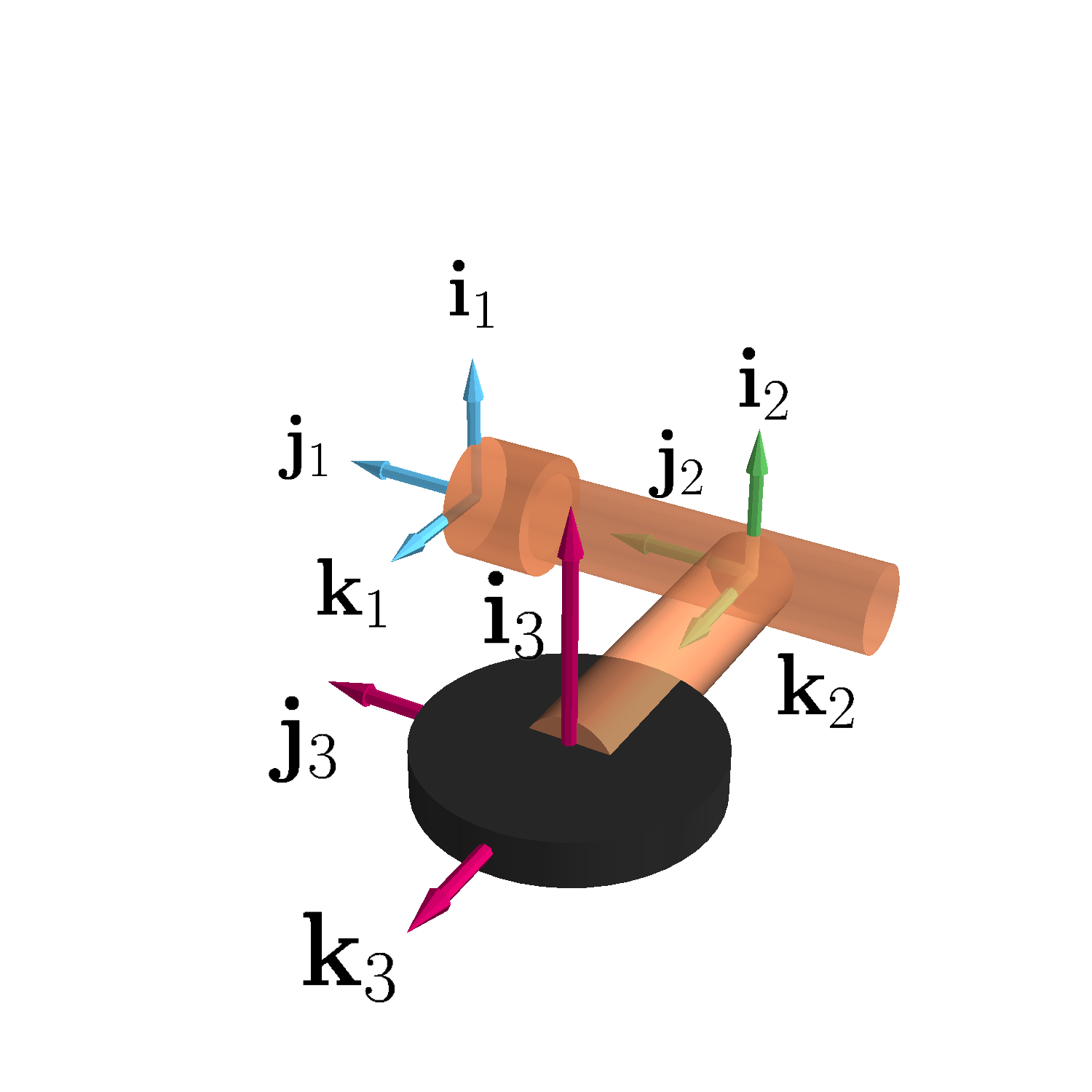
Velocity
A wheel (Frame 3) spins with angular velocity \boldsymbol\omega_3 relative to a landing gear arm (Frame 2). The landing gear arm retracts into the aircraft body (Frame 1) with angular velocity \boldsymbol\omega_2. We want to find the angular velocity of the wheel (Frame 3) relative to the aircraft body (Frame 1), denoted as \boldsymbol\omega_{3/1}.
The reference frames are:
- frame 1: Fixed to the aircraft body with unit vectors \{\mathbf i_1, \mathbf j_1, \mathbf k_1\},
- frame 2: Attached to the landing gear arm with unit vectors \{\mathbf i_2, \mathbf j_2, \mathbf k_2\},
- frame 3: Attached to the spinning wheel with unit vectors \{\mathbf i_3, \mathbf j_3, \mathbf k_3\}.
The angular velocities are:
- \boldsymbol\omega_{3/2}: angular velocity of the wheel (Frame 3) relative to the landing gear arm (Frame 2),
- \boldsymbol\omega_{2/1}: angular velocity of the landing gear arm (Frame 2) relative to the aircraft body (Frame 1),
- \boldsymbol\omega_{3/1}: angular velocity of the wheel (Frame 3) relative to the aircraft body (Frame 1).
Using the addition theorem for angular velocities:
\boldsymbol\omega_{3/1} = \boldsymbol\omega_{3/2} + \boldsymbol\omega_{2/1}
We are given \boldsymbol\omega_{3/2} = \omega_3 \mathbf i_3 (spinning of the wheel relative to Frame 2) and \boldsymbol\omega_{2/1} = \omega_2 \mathbf j_1 (retraction of the landing gear relative to Frame 1).
Due to geometry considerations, we can express both angular velocities in the same frame if we choose Frame 2.
Since \mathbf j_1 and \mathbf j_2 are always aligned, we have \boldsymbol\omega_{2/1} = \omega_2 \mathbf j_2, also since the reference frame 3 is attached to a fix arm, the \mathbf i_3 and \mathbf i_2 direction are always parallel so the rotation of frame 3 is \omega_3 \mathbf i_3 = \omega_3 \mathbf i_2.
Now we apply the addition theorem:
\boldsymbol\omega_{3/1} = \boldsymbol\omega_{3/2} + \boldsymbol\omega_{2/1} = \omega_3 \mathbf i_2 + \omega_2 \mathbf j_2
This expresses \boldsymbol\omega_{3/1} entirely in Frame 2.
To express \boldsymbol\omega_{3/1} entirely in Frame 1, we need to express the Frame 2 basis vectors (\mathbf i_2, \mathbf j_2, \mathbf k_2) in terms of the Frame 1 basis vectors (\mathbf i_1, \mathbf j_1, \mathbf k_1). The rotation of Frame 2 relative to Frame 1 is about the \mathbf j_1 axis (which is the same as \mathbf j_2) by an angle \theta = \omega_2 t:
\begin{aligned} \mathbf i_2 &= \cos(\omega_2 t) \mathbf i_1 - \sin(\omega_2 t) \mathbf k_1 \\ \mathbf j_2 &= \mathbf j_1 \\ \mathbf k_2 &= \sin(\omega_2 t) \mathbf i_1 + \cos(\omega_2 t) \mathbf k_1 \end{aligned}
Substituting the expression for \mathbf i_2 into the equation for \boldsymbol\omega_{3/1}:
\boldsymbol\omega_{3/1} = \omega_3 (\cos(\omega_2 t) \mathbf i_1 - \sin(\omega_2 t) \mathbf k_1) + \omega_2 \mathbf j_1
This simplifies to:
\boldsymbol\omega_{3/1} = \omega_3 \cos(\omega_2 t) \mathbf i_1 + \omega_2 \mathbf j_1 - \omega_3 \sin(\omega_2 t) \mathbf k_1
This final expression gives the angular velocity of the wheel (Frame 3) relative to the aircraft body (Frame 1), in terms of the fixed frame of the aircraft.
Acceleration
Let’s assume the angular velocities \omega_2 and \omega_3 are constant. We previously derived that, in reference frame 2:
\boldsymbol\omega_{3/1} = \omega_3 \mathbf i_2 + \omega_2 \mathbf j_2
Since \omega_2 and \omega_3 are constant, the relative angular accelerations \boldsymbol\alpha_{3/2} and \boldsymbol\alpha_{2/1} are zero. Using the addition theorem for angular accelerations:
\boldsymbol\alpha_{3/1} = \boldsymbol\alpha_{3/2} + \boldsymbol\alpha_{2/1} + \boldsymbol\omega_{2/1} \times \boldsymbol\omega_{3/2}
Substituting the zero angular accelerations:
\boldsymbol\alpha_{3/1} = \boldsymbol\omega_{2/1} \times \boldsymbol\omega_{3/2}
Expressing this in Frame 2:
\boldsymbol\alpha_{3/1} = (\omega_2 \mathbf j_2) \times (\omega_3 \mathbf i_2) = -\omega_2 \omega_3 \mathbf k_2
To express the angular acceleration in Frame 1, we transform -\mathbf k_2 to Frame 1:
-\mathbf k_2 = -\sin(\omega_2 t) \mathbf i_1 - \cos(\omega_2 t) \mathbf k_1
Substituting this back into the expression for \boldsymbol\alpha_{3/1}:
\boldsymbol\alpha_{3/1} = -\omega_2 \omega_3 (-\sin(\omega_2 t) \mathbf i_1 - \cos(\omega_2 t) \mathbf k_1)
Which simplifies to:
\boldsymbol\alpha_{3/1} = \omega_2 \omega_3 \sin(\omega_2 t) \mathbf i_1 + \omega_2 \omega_3 \cos(\omega_2 t) \mathbf k_1
This is the angular acceleration of Frame 3 relative to Frame 1, expressed in Frame 1.
This is an interesting result because, even with constant angular velocities, we observe a non-zero angular acceleration. This counterintuitive phenomenon is a key characteristic of three-dimensional rotational motion. This angular acceleration, as described by Euler’s second law for rotation (\mathbf{M} = I\boldsymbol\alpha), directly generates a moment. This moment, often termed the gyroscopic moment, acts on the landing gear structure. This is crucial from a design perspective because moments induce stresses and strains within the material.
In our landing gear example, this gyroscopic moment attempts to twist the landing gear assembly. If the landing gear is not designed to withstand these twisting forces, it could experience significant deformation or even failure. The magnitude of this moment is proportional to the product of the two angular velocities (\omega_2 and \omega_3), meaning that even moderately high spin rates of the wheel combined with a relatively quick retraction of the landing gear can lead to substantial gyroscopic moments and consequently, potentially damaging stresses on the structure.
This gyroscopic term arises from the fact that the direction of the angular velocity vector is changing, even if its magnitude is constant. This change in direction constitutes an angular acceleration. This moment is perpendicular to both the axis of the wheel’s spin and the axis of the landing gear’s rotation. This perpendicularity, inherent in the cross product, is the defining feature of gyroscopic effects and has significant implications in various engineering applications, from aircraft design to gyroscope navigation.
Velocity of a body wrt two reference frames
Let’s begin by expressing the position vector. We’ll consider the position from point O_1 (the origin of frame 1) to point P as follows:
\mathbf{r}_{O_1P} \big|_1 = \mathbf{r}_{O_1O_2} \big|_1 + \mathbf{r}_{O_2P} \big|_2

To determine the velocity, we need to differentiate the position vector with respect to time. Applying differentiation with respect to frame 1, we obtain:
\frac{\mathrm{d}\mathbf{r}_{O_1P}}{\mathrm{d}t} \bigg|_1 = \frac{\mathrm{d}\mathbf{r}_{O_1O_2}}{\mathrm{d}t} \bigg|_1 + \frac{\mathrm{d}\mathbf{r}_{O_2P}}{\mathrm{d}t} \bigg|_1
The left side represents the velocity of point P with respect to frame 1; the first term on the right side represents the velocity of O_2 (the origin of frame 2) with respect to frame 1, and the second term on the right represents the derivative of \mathbf{r}_{O_2P}, which is a vector expressed in the moving frame 2. We need to differentiate this vector with respect to frame 1.
Differentiating \mathbf{r}_{O_2P} \big|_2 with respect to frame 1 requires specific considerations due of the rotation of frame 2 relative to frame 1. We use the general derivative formula:
\frac{\mathrm{d}\mathbf{u}}{\mathrm{d}t} \bigg|_1 = \frac{\mathrm{d}\mathbf{u}}{\mathrm{d}t} \bigg|_2 + \boldsymbol{\omega}_{2/1} \times \mathbf{u}
where \boldsymbol{\omega}_{2/1} is the angular velocity of frame 2 relative to frame 1. Applying this formula to \mathbf{r}_{O_2P} \big|_2:
\frac{\mathrm{d}\mathbf{r}_{O_2P}}{\mathrm{d}t} \bigg|_1 = \frac{\mathrm{d}\mathbf{r}_{O_2P}}{\mathrm{d}t} \bigg|_2 + \boldsymbol{\omega}_{2/1} \times \mathbf{r}_{O_2P}\big|_2
Substituting this back into our original velocity equation:
\mathbf{v}_P \big|_1 = \mathbf{v}_{O_2} \big|_1 + \mathbf{v}_P \big|_2 + \boldsymbol{\omega}_{2/1} \times \mathbf{r}_{O_2P}\big|_2
where:
- \mathbf{v}_P \big|_1: velocity of point P with respect to frame 1 (absolute velocity),
- \mathbf{v}_{O_2} \big|_1: velocity of the origin of frame 2 (O_2) with respect to frame 1 (absolute velocity of the moving frame’s origin),
- \mathbf{v}_P \big|_2: velocity of point P with respect to frame 2 (relative velocity),
- \boldsymbol{\omega}_{2/1} \times \mathbf{r}_{O_2P}\big|_2: term accounting for the rotation of frame 2 relative to frame 1.
For brevity, we can rewrite this as:
\mathbf{v}_P = \mathbf{v}_{O_2} + \mathbf{v}_{\text{rel}} + \boldsymbol{\omega} \times \mathbf{r}
where:
- \mathbf{v}_P: absolute velocity of point P (with respect to frame 1),
- \mathbf{v}_{O_2}: absolute velocity of the origin of frame 2 (O_2) (with respect to frame 1),
- \mathbf{v}_{\text{rel}}: relative velocity of point P (with respect to frame 2),
- \boldsymbol{\omega} \times \mathbf{r}: the angular velocity of frame 2 relative to frame 1 crossed with the position vector of point P as seen in frame 2. In this case \boldsymbol{\omega} = \boldsymbol{\omega}_{2/1} and \mathbf{r} = \mathbf{r}_{O_2P}\big|_2.
This equation is valid for general three-dimensional motion and similar to the one derived for the planar case here. Unlike the planar case, \boldsymbol{\omega} is now a general vector in 3D space, not necessarily aligned with a single axis. Therefore, the cross product \boldsymbol{\omega} \times \mathbf{r} will have components in all three directions, representing the full effect of the rotation of frame 2 on the velocity of point P as observed from frame 1.
Sample problem
Let’s consider again the example of the landing gear seen previously. The gear of radius r_3 spins at an angular velocity \omega_3 and the arm rotates at angular velocity \omega_2 and the length of the arm is r_2.
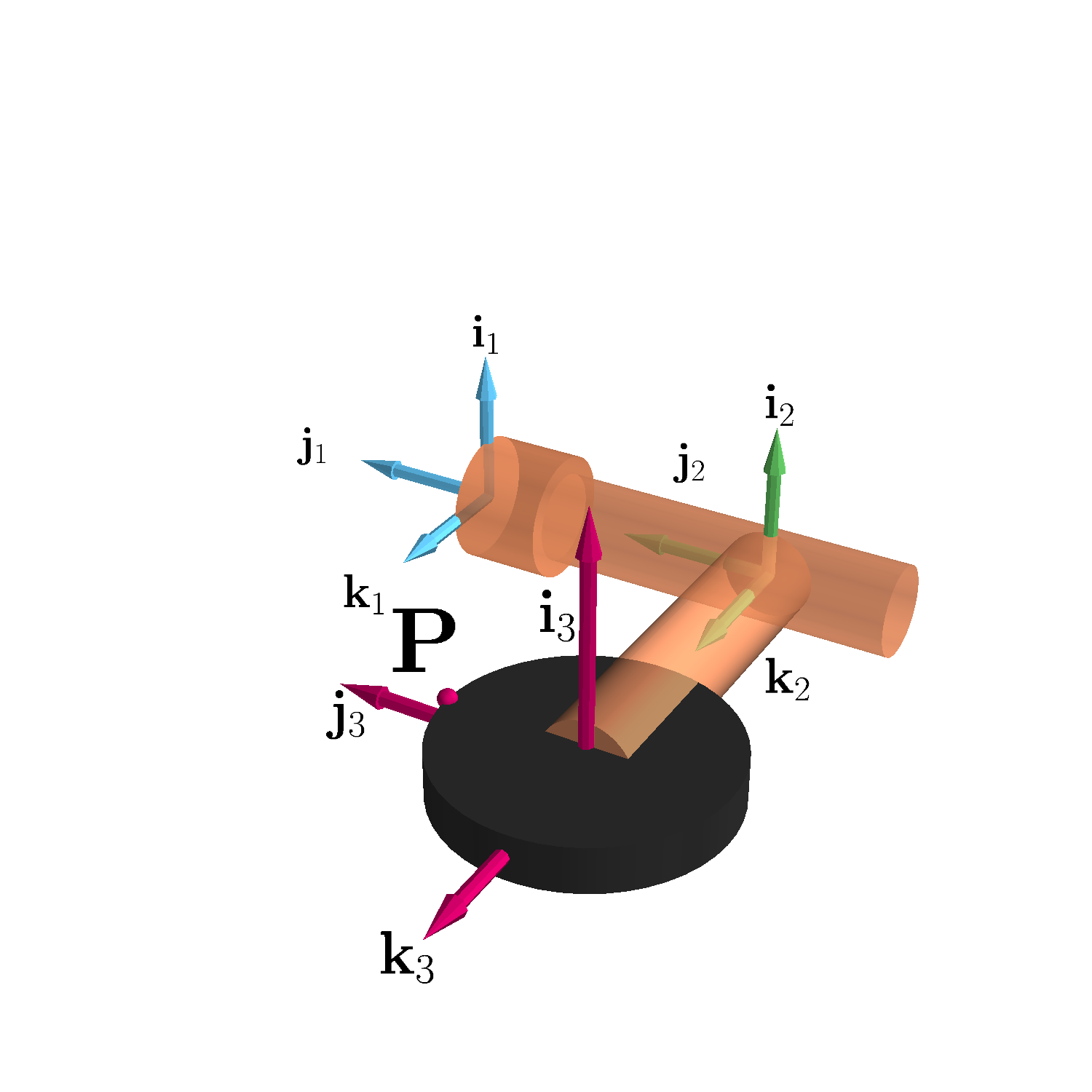
We need to find the velocity of point P on the wheel with respect to the fixed frame of reference. In the instant considered the Point P is in the \mathbf j_3 direction.
Let’s define the following reference frames:
- frame 1: fixed frame (aircraft body),
- frame 2: frame attached to the landing gear arm,
- frame 3: frame attached to the wheel
We first consider the frames 2 and 3 (considering frame 2 the fixed frame) and find the velocity of point P with respect to this fixed frame. All velocities will be put in the coordinates of frame 2:
\mathbf v_{P/2} = \mathbf v_{O_3/2} + \mathbf v_{P/3} + \boldsymbol{\omega}_{3/2} \times \mathbf r_{O_3 P/3}
where:
- \mathbf v_{P/2} is the velocity of point P with respect to frame 2,
- \mathbf v_{O_2/2} is the velocity of the origin of frame 3 with respect to frame 2,
- \mathbf v_{P/3} is the velocity of point P with respect to frame 3,
- \boldsymbol{\omega}_{3/2} is the angular velocity of frame 3 with respect to frame 2,
- \mathbf r_{O_3P/3} is the position vector from the origin of frame 3 to P.
In the problem analyzed from the perspective of frame 2 the origin of frame 3 frame is anchored in the \mathbf k_2 direction, so the velocity of the origin of the moving frames is zero (\mathbf v_{O_2/2} = 0). From the perspective of frame 3 the point is not moving, so the relative velocity is zero (\mathbf v_{P/3}=0). The angular velocity of the wheel is pointing in the \mathbf i_3 direction, but this direction is always parallel to the \mathbf i_2 direction and therefore \boldsymbol{\omega}_{3/2} = \omega_3 \mathbf i_3 = \omega_3 \mathbf i_2. Finally, \mathbf r_{O_3P/3} = r_3 \mathbf j_3 = r_3 \mathbf j_2, as the point is oriented along the \mathbf j_3 direction in that specific moment in time.
Substituting:
\mathbf v_{P/2} = \mathbf 0 + \mathbf 0 + (\omega_3 \mathbf i_2) \times (r_3 \mathbf j_2) = r_3\omega_3 \mathbf k_2
The next step is to find the velocity of point P with respect to the frame 1. We will use frame 1 as fixed and frame 2 moving. All velocities will be put in the coordinates of the frame 2:
\mathbf v_{P/1} = \mathbf v_{O_2/1} + \mathbf v_{P/2} + \boldsymbol{\omega}_{2/1} \times \mathbf r_{O_2P/2}
where:
- \mathbf v_{P/1} is the velocity of point P with respect to frame 1,
- \mathbf v_{O_2/1} is the velocity of the origin of frame 2 with respect to frame 1,
- \mathbf v_{P/2} is the velocity of point P with respect to frame 2 (calculated above),
- \boldsymbol{\omega}_{2/1} = \omega_2 \mathbf j_2 is the angular velocity of frame 2 with respect to frame 1.
- \mathbf r_{O_2P/2} = r_3 \mathbf j_2 + r_2 \mathbf k_1 is the position vector from the origin of frame 2 to point P expressed in frame 2 coordinates.
In this case also, from the perspective of the reference frame 1 the origin of frame 2 frame is anchored in the \mathbf j_2 direction, so the velocity of the origin of the moving frames is zero (\mathbf v_{O_2/1} = 0). The angular velocity is pointing in the \mathbf j_1 direction, but this direction is always parallel to the \mathbf j_2 direction and therefore \boldsymbol{\omega}_{2/1} = \omega_2 \mathbf j_1 = \omega_2 \mathbf j_2. Finally, \mathbf r_{O_2P/2} = r_3 \mathbf j_3 + r_2 \mathbf k_2 = r_3 \mathbf j_2 + r_2 \mathbf k_2, as the point is oriented along the \mathbf j_3 direction in that specific moment in time.
Substituting the known values:
\mathbf v_{P/1} = \mathbf 0 + r_3\omega_3 \mathbf k_2 + (\omega_2 \mathbf j_2) \times (r_3 \mathbf j_2 + r_2 \mathbf k_2)= r_3\omega_3 \mathbf k_2 + r_2\omega_2 \mathbf i_2
The velocity of point P with respect to the fixed frame is:
\mathbf v_{P/1} = r_2 \omega_2 \mathbf i_2 + r_3\omega_3 \mathbf k_2
This is expressed in the frame 2, but it can be transformed with geometric and kinematic consideration to a different frame.
Acceleration of a body wrt two reference frames
To find the acceleration of point \mathbf P relative to the two frames, we’ll differentiate the velocity equation with respect to time in frame 1:
\begin{aligned} \mathbf{v}_P \big|_1 &= \mathbf{v}_{O_2} \big|_1 + \mathbf{v}_P \big|_2 + \boldsymbol{\omega} \times \mathbf{r}_{O_2P}\big|_2 \\ \mathbf{a}_P \big|_1 &= \frac{\mathrm{d}\mathbf{v}_P}{\mathrm{d}t} \bigg|_1 \\ &= \frac{\mathrm{d}}{\mathrm{d}t} \left( \mathbf{v}_{O_2} \big|_1 + \mathbf{v}_P \big|_2 + \boldsymbol{\omega} \times \mathbf{r}_{O_2P}\big|_2 \right) \bigg|_1 \\ &= \frac{\mathrm{d}\mathbf{v}_{O_2}}{\mathrm{d}t} \bigg|_1 + \frac{\mathrm{d}\mathbf{v}_P}{\mathrm{d}t} \bigg|_1 + \frac{\mathrm{d}}{\mathrm{d}t} \left( \boldsymbol{\omega} \times \mathbf{r}_{O_2P} \right) \bigg|_1 \end{aligned}
where:
- \mathbf{a}_P \big|_1 is the acceleration of point P in frame 1,
- \mathbf{a}_{O_2} \big|_1= \frac{\mathrm{d}\mathbf{v}_{O_2}}{\mathrm{d}t} \big|_1 is the acceleration of the origin of frame 2 (O_2) with respect to frame 1,
- \frac{\mathrm{d}\mathbf{v}_P}{\mathrm{d}t} \big|_1 and \frac{\mathrm{d}}{\mathrm{d}t} \left( \boldsymbol{\omega} \times \mathbf{r}_{O_2P} \right) \big|_1 are the terms that require more calculations.
Using the transport theorem (derivative of a vector in different frames):
\frac{\mathrm{d}\mathbf{u}}{\mathrm{d}t} \bigg|_1 = \frac{\mathrm{d}\mathbf{u}}{\mathrm{d}t} \bigg|_2 + \boldsymbol{\omega} \times \mathbf{u}
Applying this to \frac{\mathrm{d}\mathbf{v}_P}{\mathrm{d}t} \big|_1:
\frac{\mathrm{d}\mathbf{v}_P}{\mathrm{d}t} \bigg|_1 = \frac{\mathrm{d}\mathbf{v}_P}{\mathrm{d}t} \bigg|_2 + \boldsymbol{\omega} \times \mathbf{v}_P\big|_2 = \mathbf{a}_P \big|_2 + \boldsymbol{\omega} \times \mathbf{v}_P\big|_2
Now, differentiating the term involving angular velocity:
\begin{aligned} \frac{\mathrm{d}}{\mathrm{d}t} \left( \boldsymbol{\omega} \times \mathbf{r}_{O_2P} \right)\bigg|_1 &= \frac{\mathrm{d}\boldsymbol{\omega}}{\mathrm{d}t} \bigg|_1 \times \mathbf{r}_{O_2P}\big|_2 + \boldsymbol{\omega} \times \frac{\mathrm{d}\mathbf{r}_{O_2P}}{\mathrm{d}t} \bigg|_1 \\ &= \boldsymbol{\alpha} \times \mathbf{r}_{O_2P}\big|_2 + \boldsymbol{\omega} \times \frac{\mathrm{d}\mathbf{r}_{O_2P}}{\mathrm{d}t} \bigg|_1 \end{aligned}
where \boldsymbol{\alpha} = \frac{\mathrm{d}\boldsymbol{\omega}}{\mathrm{d}t} \big|_1. Applying the transport theorem again to \frac{\mathrm{d}\mathbf{r}_{O_2P}}{\mathrm{d}t} \big|_1:
\frac{\mathrm{d}\mathbf{r}_{O_2P}}{\mathrm{d}t} \bigg|_1 = \frac{\mathrm{d}\mathbf{r}_{O_2P}}{\mathrm{d}t} \bigg|_2 + \boldsymbol{\omega} \times \mathbf{r}_{O_2P}\big|_2 = \mathbf{v}_{rel} + \boldsymbol{\omega} \times \mathbf{r}_{O_2P}\big|_2
Substituting back into the equation:
\begin{aligned} \frac{\mathrm{d}}{\mathrm{d}t} \left( \boldsymbol{\omega} \times \mathbf{r}_{O_2P} \right) \bigg|_1 &= \boldsymbol{\alpha} \times \mathbf{r}_{O_2P}\big|_2 + \boldsymbol{\omega} \times \left( \mathbf{v}_P \big|_2 + \boldsymbol{\omega} \times \mathbf{r}_{O_2P}\big|_2 \right) \\ &= \boldsymbol{\alpha} \times \mathbf{r}_{O_2P}\big|_2 + \boldsymbol{\omega} \times \mathbf{v}_P \big|_2 + \boldsymbol{\omega} \times \left( \boldsymbol{\omega} \times \mathbf{r}_{O_2P}\big|_2 \right) \end{aligned}
Finally, combining all terms:
\begin{aligned} \mathbf{a}_P \big|_1 &= \mathbf{a}_{O_2} \big|_1 + \mathbf{a}_P \big|_2 + \boldsymbol{\omega} \times \mathbf{v}_P\big|_2 + \boldsymbol{\alpha} \times \mathbf{r}_{O_2P}\big|_2 + \boldsymbol{\omega} \times \mathbf{v}_P \big|_2 + \boldsymbol{\omega} \times \left( \boldsymbol{\omega} \times \mathbf{r}_{O_2P}\big|_2 \right) \\ &= \mathbf{a}_{O_2} \big|_1 + \mathbf{a}_P \big|_2 + \boldsymbol{\alpha} \times \mathbf{r}_{O_2P}\big|_2 + 2\boldsymbol{\omega} \times \mathbf{v}_P \big|_2 + \boldsymbol{\omega} \times \left( \boldsymbol{\omega} \times \mathbf{r}_{O_2P}\big|_2 \right) \end{aligned}
Using the shorthand and dropping indexes:
\mathbf{a}_P = \mathbf{a}_{O_2} + \mathbf{a}_{\text{rel}} + \boldsymbol{\alpha} \times \mathbf{r} + 2\boldsymbol{\omega} \times \mathbf{v}_{\text{rel}} + \boldsymbol{\omega} \times (\boldsymbol{\omega} \times \mathbf{r})
where:
- \mathbf{a}_P: absolute acceleration of point P with respect to frame 1,
- \mathbf{a}_{O_2}: absolute acceleration of the origin of frame 2 with respect to frame 1,
- \mathbf{a}_{\text{rel}}: relative acceleration of point P with respect to frame 2,
- \boldsymbol{\alpha} \times \mathbf{r}: tangential acceleration of point P in frame 2,
- 2\boldsymbol{\omega} \times \mathbf{v}_{\text{rel}}: Coriolis acceleration,
- \boldsymbol{\omega} \times (\boldsymbol{\omega} \times \mathbf{r}): centripetal acceleration.
Sample problem
A vinyl record rotates with a constant angular velocity \mathbf{\omega} = \omega \mathbf{k}_2. A point P moves radially outward from the center of the record with a constant velocity \mathbf{u} = u \mathbf{i}_2 relative to the record. We need to find the velocity of point P with respect to the ground (reference frame 1).
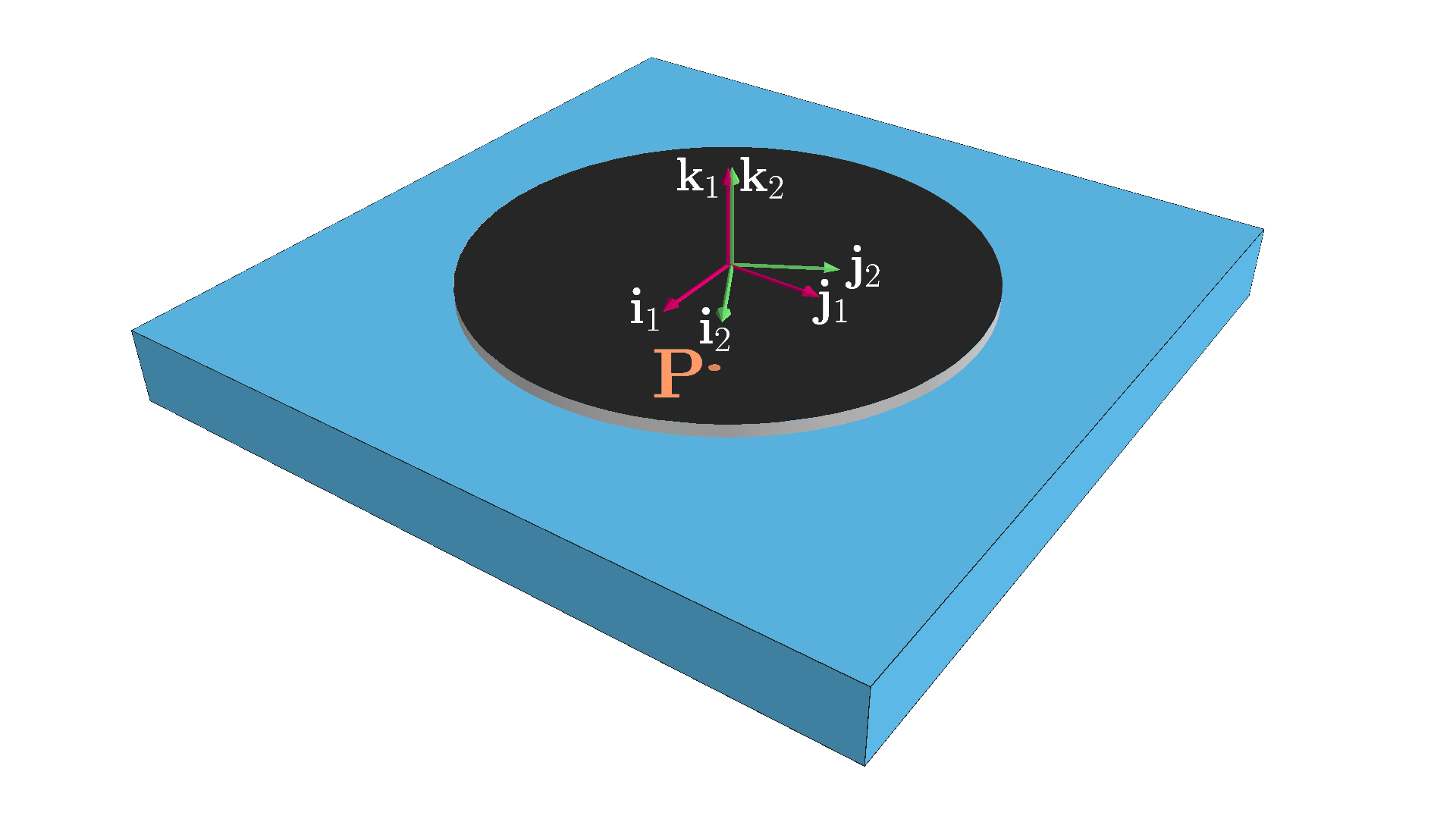
Let reference frame 1 be the ground, and reference frame 2 be the rotating record.
Velocity
The velocity of point P with respect to reference frame 1 is given by: \mathbf{v}_{P/1} = \mathbf{v}_{O_2/1} + \mathbf{v}_{P/2} + \mathbf{\omega}_{2/1} \times \mathbf{r}_{P/O_2}
- \mathbf{v}_{O_2/1} is the velocity of the origin of reference frame 2 with respect to reference frame 1, which is zero,
- \mathbf{v}_{P/2} is the velocity of P with respect to reference frame 2, which is given as u \mathbf{i}_2,
- \mathbf{\omega}_{2/1} = \omega \mathbf{k}_2 is the angular velocity of reference frame 2 with respect to reference frame 1,
- \mathbf{r}_{P/O_2} is the position vector of point P with respect to the origin of reference frame 2. If we assume the radial position of P is r then, its position is \mathbf{r}_{P/O_2} = r \mathbf{i}_2.
The velocity of point P with respect to reference frame 1 is:
\mathbf{v}_{P/1} = \mathbf{0} + u \mathbf{i}_2 + \omega \mathbf{k}_2 \times r \mathbf{i}_2= u \mathbf{i}_2 + \omega r \mathbf{j}_2
Acceleration
The acceleration of point P with respect to reference frame 1 is given by:
\mathbf{a}_{P/1} = \mathbf{a}_{O_2/1} + \mathbf{a}_{P/2} + \boldsymbol{\alpha}_{2/1} \times \mathbf{r}_{P/O_2} + 2 \boldsymbol{\omega}_{2/1} \times \mathbf{v}_{P/2} + \boldsymbol{\omega}_{2/1} \times (\boldsymbol{\omega}_{2/1} \times \mathbf{r}_{P/O_2})
- \mathbf{a}_{O_2/1} is the acceleration of the origin of reference frame 2 with respect to reference frame 1, which is zero,
- \mathbf{a}_{P/2} is the acceleration of P with respect to reference frame 2, which is zero since the velocity \mathbf{u} is constant,
- \boldsymbol{\alpha}_{2/1} is the angular acceleration of frame 2 with respect to frame 1. Since the angular velocity is constant, \boldsymbol{\alpha}_{2/1}=0,
- \mathbf{\omega}_{2/1} = \omega \mathbf{k}_2 is the angular velocity of reference frame 2 with respect to reference frame 1,
- \mathbf{v}_{P/2} is the velocity of P with respect to reference frame 2, which is u \mathbf{i}_2,
- \mathbf{r}_{P/O_2} is the position vector of point P with respect to the origin of reference frame 2. If we assume the radial position of P is r then, its position is \mathbf{r}_{P/O_2} = r \mathbf{i}_2.
Now, the acceleration of point P with respect to reference frame 1 is:
\begin{aligned} \mathbf{a}_{P/1} & = \mathbf{0} + \mathbf{0} + \mathbf{0} \times r \mathbf{i}_2 + 2 \omega \mathbf{k}_2 \times u \mathbf{i}_2 + \omega \mathbf{k}_2 \times (\omega \mathbf{k}_2 \times r \mathbf{i}_2) \\ & = 2 \omega u \mathbf{j}_2 + \omega \mathbf{k}_2 \times ( \omega r \mathbf{j}_2) \\ & = 2 \omega u \mathbf{j}_2 - \omega^2 r \mathbf{i}_2 \end{aligned}
The acceleration of point P with respect to the ground (reference frame 1) consists of two components: the centripetal acceleration and the Coriolis acceleration.
The centripetal acceleration term is -\omega^2 r \mathbf{i}_2. This term arises due to the rotation of the moving reference frame (frame 2). If the point P had no radial velocity relative to the rotating frame (i.e., \mathbf{u} = 0), then this term would be the only acceleration that the point would experience with respect to the ground. This acceleration is always directed towards the center of rotation. The magnitude of this acceleration is \omega^2 r.
The Coriolis acceleration term is 2 \omega u \mathbf{j}_2. This term arises when a point moves with a velocity relative to a rotating reference frame, and it is perpendicular to the radial velocity. It is the result of the combined effect of the rotation of the reference frame and the point’s motion within that frame:
- if the point has no radial relative velocity, the Coriolis acceleration is zero,
- if the point has a radial relative velocity, it will experience a Coriolis acceleration that is perpendicular to the velocity \mathbf u, and also perpendicular to the rotation axis,
- if the motion of the point were frictionless, the moving frame would move underneath the point with relative radial velocity \mathbf u and the point would go straight, but due to the effect of Coriolis the point is accelerated tangentially, meaning that it appears to be deviated with respect to the inertial frame.